Survival Extrapolation (Parametric Models)
Fits candidate parametric survival models to the observed follow-up and projects them beyond the data to the lifetime horizon — the central, high-leverage step of any HTA survival model.
When an economic model needs lifetime survival but the data end at a few years (the usual case). Per NICE DSU TSD 14, fit a slate of parametric families, judge fit within the data AND clinical plausibility of the tail, and carry the choice into scenario analysis.
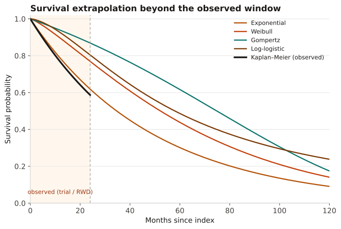
Inside the observed window all curves track the KM; beyond it they diverge sharply — the tail you pick drives lifetime QALYs and the ICER. Never report a single extrapolation without alternatives as scenarios.
Kaplan–Meier is observed to 24 months; exponential, Weibull, Gompertz, and log-logistic models are fit to that window and extrapolated to 120 months. The shaded region marks the observed data; the curves diverge in the unobserved tail.
Result: All four fit the observed window similarly but diverge after 24 months: at 120 months survival ranges from ~5% (Gompertz) to ~25% (log-logistic). Restricted mean survival over the horizon differs by >1 year across families — so the extrapolation choice is itself a headline driver and must be a scenario in the economic model.
Reference: Latimer NR. Survival analysis for economic evaluations alongside clinical trials — extrapolation with patient-level data (NICE DSU TSD 14). Med Decis Making. 2013;33(6):743-754.