Disease Risk Scores

In plain language

A disease risk score (DRS) is a single number that captures how likely a patient is to have the outcome based on their baseline health, before considering the drug being studied. You build it by fitting a model that predicts the outcome from background characteristics (usually in patients who did not take the drug), then giving every patient a score. Comparing treated and untreated patients who share the same score controls many confounders at once - and it works even when very few people took the drug or the drug is brand new, situations where the more common propensity score struggles. The catch: the score is only as good as the outcome model behind it, so a wrong model or one fit in the wrong group of patients quietly leaves confounding behind.

A disease risk score (DRS) collapses a long list of baseline confounders into a single number: each patient's predicted probability (or hazard) of the outcome in the absence of the exposure of interest. Where a propensity score models the exposure (probability of getting the drug given covariates), a DRS models the outcome (probability of the event given covariates) - it is, in Hansen's phrase, the prognostic analogue of the propensity score. You fit an outcome-prediction model, read off each person's baseline risk, and then control confounding by stratifying, matching, or regression-adjusting on that one score instead of on the raw covariates. Two patients with the same DRS have the same baseline prognosis, so comparing the exposed and the unexposed within a DRS stratum removes the confounding those covariates carried.

Core conceptual distinction - where the model is fit

This is the decision that makes or breaks a DRS. - Unexposed-only (reference-population) DRS: Fit the outcome model among the unexposed (the comparator or background population), then score everyone, including the exposed. This is the original Hansen construction. It cannot bake the exposure effect into the score, so it does not "adjust away" a real effect - but it assumes the covariate-outcome relationships estimated in the unexposed transport to the exposed. - Full-cohort DRS: Fit the outcome model in the whole cohort with an exposure term included, then set the exposure term to "unexposed" for everyone when predicting. Statistically efficient, but it borrows the exposed patients' outcomes to estimate the score, risking a subtle form of overfitting-to-the-effect and constraining the exposure-outcome relationship to the model's form. 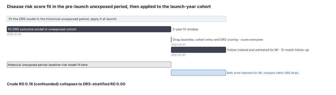- Historical-period DRS: Fit the model in a historical cohort from before the drug existed (or before a formulary change), then apply it to the current cohort. This is the move that rescues studies of new market entrants - a just-launched drug has no historical users, so you cannot build a propensity model that separates its users from comparators, but you can build an outcome model in the pre-launch era and carry it forward. The cost is calendar drift: secular changes in coding, treatment, and baseline risk can make a historical score miscalibrated for the present.

Pros, cons, and trade-offs

(specific and comparative). - vs propensity-score-methods-psm-iptw (the main alternative): The classic asymmetry is exposure prevalence vs outcome frequency. A propensity score is hard to estimate well when exposure is rare (few exposed patients to model who gets the drug) but easy when the outcome is rare; a DRS is the mirror image - it is hard to estimate when the outcome is rare (few events to fit the risk model) but thrives when the outcome is common and exposure is rare. So prefer a DRS for a rare exposure with a common outcome; prefer a propensity score for a common exposure with a rare outcome. The other decisive DRS advantage is the new-drug / no-exposure-history case above, where a propensity model literally cannot be fit. - vs high-dimensional-propensity-score-hdps-rwe: hdPS is a propensity-side, data-adaptive way to surface hundreds of proxy confounders from claims; a DRS is an outcome-side single summary. They are not rivals - you can build a high-dimensional disease risk score with the same proxy-selection machinery on the outcome model. The trade-off is the same exposure-vs-outcome-frequency one, plus DRS's reliance on getting the outcome model's functional form right. - vs traditional multivariable outcome regression: A DRS is essentially a two-stage version of outcome regression - fit the covariate-outcome model once, then condition the exposure contrast on its single output. The practical pay-offs are a clean separation of the confounder model from the effect estimate (you can inspect DRS overlap before ever looking at the exposure effect, reducing the temptation to fish), parsimony when covariates vastly outnumber events, and a transparent diagnostic (DRS distribution by exposure). In large simulations the three approaches perform comparably when correctly specified; DRS's edge is operational, not a magic bias reducer.

When to use

Reach for a DRS when (1) the exposure is rare and the outcome is common, so there is plenty of outcome signal to fit a risk model but too few exposed to fit a stable propensity model; (2) you are studying a newly launched drug or new market entrant with no historical exposure to model - fit the outcome model in the pre-launch/unexposed era and carry it forward; (3) you have multiple exposures or comparators sharing one outcome - one DRS can be reused across exposure contrasts, whereas each contrast needs its own propensity model; (4) you want a confounder summary you can lock down and inspect before unblinding the exposure effect.

When NOT to use - and when it is actively misleading

- Rare outcome. With few events, the outcome model is unstable and overfit; the DRS inherits that noise. Here a propensity score (modeling the abundant exposure signal) is the better tool. Do not force a DRS onto a rare-event study just to avoid a propensity model. - Outcome-model misspecification. A DRS is only as good as the risk model behind it. If the functional form is wrong (omitted interactions, wrong link, miscaptured non-linearity), residual confounding leaks through even after you stratify on the score - and unlike a propensity score, you cannot diagnose it by checking covariate balance across exposure groups, because the DRS is not built to balance covariates by exposure. Check balance and DRS overlap explicitly. - Fitting in the wrong population (the most dangerous trap). If you fit a full-cohort DRS with the exposed included and let the model see the exposure's effect, the score can partially absorb a true exposure effect, biasing the contrast toward the null. And if you fit an unexposed-only or historical DRS in a population whose covariate-outcome relationships do not transport to the exposed (different era, different case mix, calendar drift in coding), the score is miscalibrated and residual confounding returns. Always pre-specify the fitting population, and sanity-check the historical or unexposed model's calibration in the target cohort.

Data-source operational depth

In claims the DRS outcome model is typically a logistic or Cox model built from baseline diagnoses, procedures, drugs, demographics, and prior utilization in the pre-index window; the standard immortal-time and look-back hygiene of any new-user design applies (covariates must be measured before the index date, never after). In EHR richer predictors (labs, vitals, smoking, BMI) usually make the outcome model far better calibrated than a claims-only DRS, which is the whole game for a method that lives or dies by outcome-model quality. Registry data can supply adjudicated outcomes and a clean reference cohort for fitting. Linked claims-EHR is the ideal substrate: EHR for the predictors that calibrate the risk model, claims for complete capture of the (common) outcome events and follow-up.

Interpreting the output

Using the worked example above: the crude comparison yields a risk difference of 0.33 − 0.17 = 0.16 (treated patients appear to have higher MI risk). DRS stratification collapses this to a pooled risk difference of 0.00.

Formal interpretation: The crude risk difference of 0.16 reflects confounding by baseline prognosis — treated patients were concentrated in the high-risk DRS band (score ≈ 0.35), where MI rates were naturally elevated. Within each DRS stratum, the treated–untreated risk difference is 0.50 − 0.50 = 0.00 in the high-risk band and 0 − 0 = 0.00 in the low-risk band. The DRS-stratified pooled risk difference of 0.00 estimates the treatment effect conditional on baseline prognostic risk — among patients for whom comparable baseline prognosis exists in both treatment arms. This is a valid causal estimate under the assumption that the DRS outcome model is correctly specified in the unexposed reference population and that no unmeasured confounding remains after conditioning on baseline risk strata. Unlike propensity score methods, DRS adjustment does not require a well-specified exposure model, but it does require a well-calibrated outcome model.

Practical interpretation: Once patients with similar underlying heart attack risk are compared within the same stratum, the drug shows no excess MI risk — the apparent harm in the crude analysis was entirely driven by sicker patients being disproportionately in the treated group. The DRS adjustment is especially useful when exposure is rare and a propensity score model would be unstable, because the risk model is estimated in the more numerous unexposed population.

Worked example

Scenario

A drug launches and only a handful of patients take it in its first year, but the outcome we care about (a heart attack, MI) is common. A propensity score would struggle because exposure is so rare, so we use a disease risk score instead. We fit a model that predicts MI from baseline characteristics among the untreated patients, give every patient a baseline-risk score, then split patients into a high-risk and a low-risk band and compare treated versus untreated MI rates within each band. We have 12 patients: 6 treated and 6 untreated.

Dataset

One row per patient. drs is the model-predicted baseline MI risk; mi_event is 1 if the patient had an MI in follow-up.

Steps

• The outcome model fit among the untreated gives each patient a baseline MI risk - a patient with diabetes and a prior MI scores higher (about 0.35) than a patient with neither (about 0.10); these predicted risks are the drs column.

• Crude (unadjusted) comparison ignoring the score - treated MI risk = 2/6 = 0.33, untreated MI risk = 1/6 = 0.17, so the crude risk difference = 0.33 - 0.17 = 0.16, making the drug look harmful.

• Split on the DRS into a high-risk band (drs 0.35, patients 1-6) and a low-risk band (drs 0.10, patients 7-12).

• High-risk band - treated MI risk = 2/4 = 0.50, untreated MI risk = 1/2 = 0.50, so the within-band risk difference = 0.50 - 0.50 = 0.00.

• Low-risk band - treated MI risk = 0/2 = 0, untreated MI risk = 0/4 = 0, so the within-band risk difference is also 0.

• Pool the two bands weighted by their size (6 of 12 each, weight 0.5) - pooled DRS-adjusted risk difference = 0.5 0.00 + 0.5 0.00 = 0.00.

Result

The crude risk difference of 0.16 made the drug look harmful, but that was confounding - the treated patients were concentrated in the high baseline-risk band. After stratifying on the disease risk score, the pooled risk difference is 0.00, showing no effect once baseline prognosis is matched.

Timeline Spec

Title

Disease risk score fit in the pre-launch unexposed period, then applied to the launch-year cohort

Window

Start

2018-01-01

End

2021-12-31

Label

Fit the DRS model in the historical unexposed period, apply it at launch

Events

• Label

  Fit DRS outcome model in unexposed cohort

  Start

  2018-01-01

  Length Days

  1095

  Quantity

  3-year fit window

• Label

  Drug launches; cohort entry and DRS scoring

  Start

  2021-01-01

  Length Days

  1

  Quantity

  score everyone

• Label

  Follow treated and untreated for MI

  Start

  2021-01-01

  Length Days

  365

  Quantity

  12-month follow-up

Spans

• Kind

  unexposed

  Start

  2018-01-01

  End

  2020-12-31

  Label

  Historical unexposed period: baseline-risk model fit here

• Kind

  followup

  Start

  2021-01-01

  End

  2021-12-31

  Label

  Both arms followed for MI; compare within DRS strata

Result

Label

Crude RD 0.16 (confounded) collapses to DRS-stratified RD 0.00

Runnable example

import numpy as np
import pandas as pd
import statsmodels.api as sm

def disease_risk_score(df, outcome, exposure, covariates, n_strata=5):
    # 1) Fit the outcome model among the UNEXPOSED only (no exposure term) -> baseline risk model.
    ref = df[df[exposure] == 0]
    drs_model = sm.Logit(ref[outcome], sm.add_constant(ref[covariates])).fit(disp=0)

    # 2) Score EVERYONE (exposed included) with that model: DRS = predicted baseline risk.
    X_all = sm.add_constant(df[covariates], has_constant="add")
    df = df.assign(drs=np.asarray(drs_model.predict(X_all)))

    # 3) Stratify on the DRS and take a stratum-weighted exposed-vs-unexposed risk difference.
    df = df.assign(stratum=pd.qcut(df["drs"], n_strata, labels=False, duplicates="drop"))
    rows = []
    for s, g in df.groupby("stratum"):
        e = g.loc[g[exposure] == 1, outcome]
        u = g.loc[g[exposure] == 0, outcome]
        if len(e) and len(u):                       # both arms present (DRS positivity)
            rows.append({"stratum": s, "n": len(g), "rd": e.mean() - u.mean()})
    strata = pd.DataFrame(rows)
    w = strata["n"] / strata["n"].sum()
    pooled_rd = float((w * strata["rd"]).sum())
    return pooled_rd, strata, drs_model

disease_risk_score <- function(df, outcome, exposure, covariates, n_strata = 5) {
  # 1) Fit the outcome (baseline risk) model among the UNEXPOSED only.
  ref  <- df[df[[exposure]] == 0, ]
  form <- as.formula(paste(outcome, "~", paste(covariates, collapse = " + ")))
  drs_model <- glm(form, data = ref, family = binomial())

  # 2) Score EVERYONE with that model: DRS = predicted baseline risk.
  df$drs <- predict(drs_model, newdata = df, type = "response")

  # 3) Stratify on the DRS (quantile cut) and pool within-stratum risk differences.
  brks <- quantile(df$drs, probs = seq(0, 1, length.out = n_strata + 1), na.rm = TRUE)
  df$stratum <- cut(df$drs, breaks = unique(brks), include.lowest = TRUE, labels = FALSE)
  agg <- do.call(rbind, lapply(split(df, df$stratum), function(g) {
    e <- g[g[[exposure]] == 1, outcome]
    u <- g[g[[exposure]] == 0, outcome]
    if (length(e) > 0 && length(u) > 0)            # both arms present (DRS positivity)
      data.frame(stratum = g$stratum[1], n = nrow(g), rd = mean(e) - mean(u))
    else NULL
  }))
  w <- agg$n / sum(agg$n)
  list(pooled_rd = sum(w * agg$rd), strata = agg, model = drs_model)
}