Distributional Cost-Effectiveness Analysis

In plain language

Distributional cost-effectiveness analysis (DCEA) asks not just whether a health program is good value on average, but who gains and who loses - splitting the population into groups we have fairness concerns about (such as poorer vs richer areas, or by race) and tracking how much health each group ends up with. It adds up health the program creates, subtracts the health lost elsewhere because the money had to come from somewhere, and then scores the result with a dial called inequality aversion: turn the dial up and gains to the worse-off count for more. The payoff is a single honest picture of the trade-off between making total health bigger and making it more equal, instead of averaging that tension away.

Standard cost-effectiveness analysis (CEA) and cost-utility analysis (CUA) ask one question: does the intervention buy more health (QALYs) than the next-best use of the same money? They answer it for the average patient and are deliberately blind to who gains and who loses. Distributional cost-effectiveness analysis (DCEA) keeps the efficiency question but adds a second one society actually cares about: how is that net health benefit distributed across groups we have equity concerns about - the most-deprived vs the least-deprived fifth of an area-deprivation index, Black vs White patients, rural vs urban populations - and is the program worth adopting once we weight gains to the worse-off more heavily than gains to the better-off? DCEA does this by (1) estimating the baseline distribution of lifetime health (quality-adjusted life expectancy) across subgroups, (2) estimating the net health benefit each subgroup gets from the intervention - health gained minus health displaced elsewhere by the opportunity cost of spending - (3) adding the net benefit onto the baseline to get the post-intervention distribution, and (4) collapsing each distribution to a single number with a social welfare function that embeds an inequality-aversion parameter (the Atkinson epsilon). The decision then turns on the equity-weighted health, not the unweighted total.

Core conceptual machinery

Three pieces must be pre-specified. (1) The equity-relevant subgroups and the baseline distribution: you cannot weight a distribution you have not measured, so DCEA needs subgroup-specific baseline health (e.g., quality-adjusted life expectancy by deprivation quintile). (2) The opportunity cost and its incidence: a fixed budget means funding a new program displaces health somewhere else; that displaced health (cost divided by the cost-effectiveness threshold k) must be subtracted, and crucially the displacement may fall on different groups than the gains - a program that helps the deprived but is financed by cuts that also hit the deprived can be equity-neutral or worse. (3) The social welfare function and the inequality-aversion parameter: the Atkinson equally distributed equivalent (EDE) is the level of health which, if everyone had it equally, would be judged exactly as good as the actual unequal distribution. As epsilon rises from 0 (pure efficiency, EDE = mean) the EDE bends below the mean and the analysis pays more for equality. The headline output is the equity-weighted net benefit = change in EDE, set against the unweighted net benefit = change in the mean. When the two point the same way the decision is easy; when they conflict you are on the equity-efficiency trade-off plane and the decision is a value judgment DCEA makes transparent rather than hides.

Two flavors that differ in data demand

Equity impact analysis maps where the gains and losses land - the pure distributional picture - without committing to a single inequality-aversion number; it answers who benefits. Equity-weighted (full) DCEA goes the extra step of running the social welfare function at one or more epsilon values to produce an adopt/reject verdict. You can report the first without the second, and reasonable analysts often do, because choosing epsilon is contestable.

Pros, cons, and trade-offs

(specific and comparative). - vs cost-effectiveness / cost-utility analysis (the parent): DCEA contains CEA as the special case epsilon = 0 (no inequality aversion - the EDE collapses to the mean and you are back to maximizing total QALYs). Its value-add is making the distribution and the equity weighting explicit, so a program that improves average health while widening the health gap can be flagged rather than rubber-stamped. Prefer plain CEA/CUA when there is no credible equity concern, no subgroup heterogeneity in effect or baseline health, or no data to characterize the distribution; the extra machinery then adds assumptions without changing the answer. - vs subgroup CEA (running a separate ICER per group): Subgroup CEA tells you the cost-effectiveness within each group but never combines them into a single equity-aware verdict and ignores the opportunity-cost incidence across groups. DCEA's social welfare step is exactly the aggregation subgroup CEA refuses to do. Prefer subgroup CEA only as a descriptive precursor. - vs the aggregate DCEA shortcut: Full DCEA needs subgroup-specific effectiveness, costs, and baseline health - often unavailable. The aggregate DCEA shortcut combines the overall (non-distributional) cost-effectiveness result with external data on how the disease and the opportunity cost are socially distributed to approximate the equity impact at far lower data cost. Prefer aggregate DCEA for early or data-poor appraisals; prefer full DCEA when subgroup RWD can support patient-level distributional estimates.

When to use

When equity is an explicit objective of the decision-maker (many HTA bodies now ask for it); when the intervention plausibly has different effectiveness, uptake, adherence, or baseline risk across deprivation, race/ethnicity, or geography; when the financing of the program (and thus its opportunity cost) lands disproportionately on a group; when two options have similar ICERs but different distributional footprints and the tie should be broken on equity; and when real-world data let you estimate subgroup-specific effectiveness and costs that a trial's narrow population cannot.

When NOT to use - and when it is actively misleading

- No real distributional signal. If baseline health, effect, and costs are genuinely homogeneous across groups, DCEA's EDE moves in lockstep with the mean and the equity weighting is decorative - it manufactures an appearance of equity analysis while changing nothing. Do not dress a standard CUA in DCEA clothing to satisfy a checkbox. - Subgroups built from biased real-world data. DCEA inherits every confounding and measurement problem of the underlying RWE: if the subgroup-specific effectiveness estimates are confounded (deprived patients differ in severity, adherence, and competing risks), the distribution you weight is wrong, and a confident equity verdict rests on a biased input. Race/ethnicity and deprivation are often mismeasured or missing in claims, so the subgroups themselves can be misclassified. - Ignoring the opportunity-cost incidence. Counting only who gains and assuming the displaced health is spread evenly (or ignoring it) systematically flatters programs financed by cutting services the deprived rely on. The net-benefit subtraction and its group incidence are not optional - omitting them is the most common way DCEA overstates pro-equity impact. - Treating epsilon as a fact. The inequality-aversion parameter is a social value, not an estimate. Reporting a single epsilon as if it were measured, with no sensitivity analysis across the plausible range, hides the very value judgment DCEA exists to surface. Always sweep epsilon and show where the verdict flips.

Data-source operational depth

DCEA's distinctive demand is subgroup-specific everything: effectiveness, costs, baseline health, and a credible equity stratifier, ideally all on the same population. Real-world data are where those subgroup estimates can actually be built (trials rarely carry deprivation or race with enough power), but the equity stratifier and the subgroup effect estimates are exactly the fields most fragile in routine data. The aggregate-DCEA shortcut exists precisely because the full subgroup matrix is so often unavailable.

Worked intuition

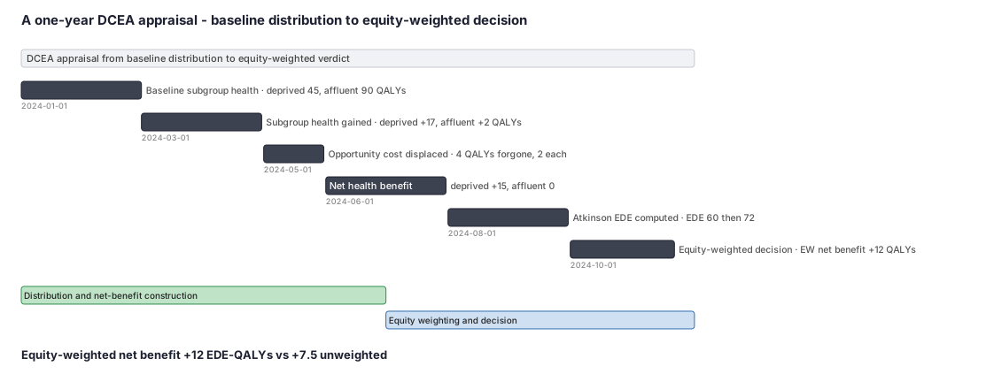
Split a population into a more-deprived and a less-deprived half with baseline quality-adjusted life expectancies of 45 and 90 QALYs. A program delivers 17 QALYs of health to the deprived half and 2 to the affluent half; financing it displaces 4 QALYs of health (cost / threshold), falling 2 on each half. Net benefit is thus +15 to the deprived half and 0 to the affluent half. Average health rises from 67.5 to 75 QALYs (+7.5, the ordinary CEA signal), but because the gains are pro-poor, the Atkinson EDE (epsilon = 2) rises from 60 to 72 - an equity-weighted net benefit of +12, larger than the +7.5 unweighted gain. A more efficient alternative that pushed average health higher while routing the gains to the already-healthy could show the opposite: a bigger mean uplift but a smaller (or negative) EDE change. That divergence is the entire point of DCEA.

Interpreting the output

Consider the worked example: the program produces an unweighted average gain of 7.5 QALYs but an equity-weighted net benefit of +12 EDE-QALYs, and the Atkinson inequality index falls from 0.111 to 0.04.

Formal interpretation: The EDE-QALY gain of 12 is the change in the equally distributed equivalent health — the level of equal health that the social welfare function (with inequality aversion parameter epsilon = 2) regards as equivalent to the actual unequal post-intervention distribution. It exceeds the average gain of 7.5 because the program's benefits are concentrated in the worse-off group, and the Atkinson social welfare function penalizes inequality, so reducing it earns an equity premium. The Atkinson index of 0.111 before the intervention means 11.1% of average health is wasted by inequality; after the program it falls to 4%. These numbers are conditional on the choice of epsilon: a higher inequality-aversion parameter would widen the gap between 12 and 7.5; a lower one would narrow it toward the ordinary CEA signal. The choice of epsilon is a value judgment that must be made explicit and varied in sensitivity analysis.

Practical interpretation: The equity-efficiency trade-off DCEA reveals is that a more efficient alternative routing gains to the already-healthy could produce a larger average QALY gain but a smaller EDE improvement. Report both the unweighted QALY gain and the equity-weighted EDE gain side by side, with at minimum two epsilon values (e.g., 1 and 2), so decision-makers can see how much of the apparent advantage depends on the inequality-aversion assumption. A DCEA verdict of "favorable" can reverse to "unfavorable" when epsilon changes — that instability is the output, not a limitation to hide.

Worked example

Scenario

A health system is deciding whether to fund a new program and wants an equity-aware answer, not just an average one. It splits the population into two equal halves - a more-deprived half and a less-deprived half - whose baseline quality-adjusted life expectancies are 45 and 90 QALYs. The program delivers health to both halves but is paid for out of a fixed budget, so some health is displaced elsewhere. We compute the ordinary average gain and the equity-weighted gain (using an inequality-aversion dial of epsilon = 2) and compare them.

Dataset

The subgroup inputs an analyst would assemble for a two-group DCEA (one row per equity subgroup).

Steps

• Find the opportunity-cost displacement from the budget constraint. The program costs $80,000 and the threshold is $20,000 per QALY, so health displaced elsewhere = $80,000 / $20,000 = 4 QALYs, split 2 and 2 across the halves.

• Net health benefit per subgroup = health gained minus displacement. More-deprived = 17 - 2 = 15 QALYs; less-deprived = 2 - 2 = 0 QALYs.

• Post-intervention health = baseline plus net benefit. More-deprived = 45 + 15 = 60; less-deprived = 90 + 0 = 90.

• Ordinary CEA signal = change in average health. Baseline mean = (45 + 90) / 2 = 67.5; post mean = (60 + 90) / 2 = 75; unweighted net benefit = 75 - 67.5 = 7.5 QALYs.

• Equity-weighting uses the Atkinson equally distributed equivalent (EDE); at epsilon = 2 the EDE is the harmonic mean = 2 divided by the sum of reciprocals. Baseline EDE = 2 / (1/45 + 1/90) = 60; post EDE = 2 / (1/60 + 1/90) = 72.

• Equity-weighted net benefit = change in EDE = 72 - 60 = 12 QALYs, which is larger than the 7.5 unweighted gain because the program's health went mostly to the worse-off half.

• Inequality also fell. Atkinson index = 1 minus EDE over mean; before = 1 - 60 / 67.5 = 0.111, after = 1 - 72 / 75 = 0.04 - the health gap narrowed.

Result

The program raises average health by 7.5 QALYs but, because the gains are pro-poor, its equity-weighted net benefit is +12 EDE-QALYs (the equity premium is 12 - 7.5 = 4.5), and the Atkinson inequality index falls from 0.111 to 0.04. A more efficient alternative that routed gains to the already-healthy half could show a bigger mean uplift but a smaller EDE change - the equity-efficiency trade-off DCEA exists to reveal.

Timeline Spec

Title

A one-year DCEA appraisal - baseline distribution to equity-weighted decision

Window

Start

2024-01-01

End

2024-12-01

Label

DCEA appraisal from baseline distribution to equity-weighted verdict

Events

• Label

  Baseline subgroup health

  Start

  2024-01-01

  Length Days

  60

  Quantity

  deprived 45, affluent 90 QALYs

• Label

  Subgroup health gained

  Start

  2024-03-01

  Length Days

  60

  Quantity

  deprived +17, affluent +2 QALYs

• Label

  Opportunity cost displaced

  Start

  2024-05-01

  Length Days

  30

  Quantity

  4 QALYs forgone, 2 each

• Label

  Net health benefit

  Start

  2024-06-01

  Length Days

  60

  Quantity

  deprived +15, affluent 0

• Label

  Atkinson EDE computed

  Start

  2024-08-01

  Length Days

  60

  Quantity

  EDE 60 then 72

• Label

  Equity-weighted decision

  Start

  2024-10-01

  Length Days

  52

  Quantity

  EW net benefit +12 QALYs

Spans

• Kind

  exposed

  Start

  2024-01-01

  End

  2024-06-30

  Label

  Distribution and net-benefit construction

• Kind

  followup

  Start

  2024-07-01

  End

  2024-12-01

  Label

  Equity weighting and decision

Result

Label

Equity-weighted net benefit +12 EDE-QALYs vs +7.5 unweighted

Value

12

Runnable example

from typing import Sequence

def atkinson_ede(health: Sequence[float], shares: Sequence[float], epsilon: float) -> float:
    # Equally distributed equivalent: the equal level of health judged as good as the actual distribution.
    # epsilon = 0 -> mean (pure efficiency); epsilon -> larger weights the worse-off more.
    tot = sum(shares)
    w = [s / tot for s in shares]
    if abs(epsilon - 1.0) < 1e-9:                      # limiting case: weighted geometric mean
        import math
        return math.exp(sum(wi * math.log(hi) for wi, hi in zip(w, health)))
    s = sum(wi * hi ** (1.0 - epsilon) for wi, hi in zip(w, health))
    return s ** (1.0 / (1.0 - epsilon))

def atkinson_index(health, shares, epsilon):
    mean = sum(s * h for s, h in zip(shares, health)) / sum(shares)
    return 1.0 - atkinson_ede(health, shares, epsilon) / mean

def dcea(baseline, shares, health_gained, opp_cost_displaced, epsilon):
    # Net health benefit per subgroup = health gained - opportunity-cost displacement.
    nhb  = [g - d for g, d in zip(health_gained, opp_cost_displaced)]
    post = [b + n for b, n in zip(baseline, nhb)]
    mean0 = sum(s * h for s, h in zip(shares, baseline)) / sum(shares)
    mean1 = sum(s * h for s, h in zip(shares, post)) / sum(shares)
    ede0  = atkinson_ede(baseline, shares, epsilon)
    ede1  = atkinson_ede(post, shares, epsilon)
    return {
        "net_health_benefit": nhb,
        "unweighted_net_benefit": round(mean1 - mean0, 4),   # ordinary CEA signal
        "equity_weighted_net_benefit": round(ede1 - ede0, 4),
        "atkinson_index_before": round(atkinson_index(baseline, shares, epsilon), 4),
        "atkinson_index_after": round(atkinson_index(post, shares, epsilon), 4),
    }

if __name__ == "__main__":
    # Two equal halves: more-deprived (45 QALYs) and less-deprived (90 QALYs).
    baseline = [45.0, 90.0]
    shares   = [0.5, 0.5]
    gained   = [17.0, 2.0]    # health the program delivers to each half
    opp_cost = [2.0, 2.0]     # displaced health: total cost / threshold = 4 QALYs, split evenly
    print(dcea(baseline, shares, gained, opp_cost, epsilon=2.0))
    # -> unweighted +7.5, equity-weighted +12.0, Atkinson index 0.1111 -> 0.04

atkinson_ede <- function(health, shares, epsilon) {
  w <- shares / sum(shares)
  if (abs(epsilon - 1) < 1e-9) {                 # limiting case: weighted geometric mean
    return(exp(sum(w * log(health))))
  }
  s <- sum(w * health^(1 - epsilon))
  s^(1 / (1 - epsilon))
}

atkinson_index <- function(health, shares, epsilon) {
  mean_h <- sum(shares * health) / sum(shares)
  1 - atkinson_ede(health, shares, epsilon) / mean_h
}

dcea <- function(baseline, shares, health_gained, opp_cost_displaced, epsilon) {
  nhb  <- health_gained - opp_cost_displaced     # net health benefit per subgroup
  post <- baseline + nhb
  mean0 <- sum(shares * baseline) / sum(shares)
  mean1 <- sum(shares * post)     / sum(shares)
  ede0  <- atkinson_ede(baseline, shares, epsilon)
  ede1  <- atkinson_ede(post,     shares, epsilon)
  list(
    net_health_benefit          = nhb,
    unweighted_net_benefit      = round(mean1 - mean0, 4),   # ordinary CEA signal
    equity_weighted_net_benefit = round(ede1 - ede0, 4),
    atkinson_index_before       = round(atkinson_index(baseline, shares, epsilon), 4),
    atkinson_index_after        = round(atkinson_index(post,     shares, epsilon), 4)
  )
}

# Two equal halves: more-deprived (45 QALYs) and less-deprived (90 QALYs).
baseline <- c(45, 90); shares <- c(0.5, 0.5)
gained   <- c(17, 2)            # health delivered to each half
opp_cost <- c(2, 2)             # displaced health: total cost / threshold = 4 QALYs, split evenly
print(dcea(baseline, shares, gained, opp_cost, epsilon = 2))
# -> unweighted +7.5, equity-weighted +12, Atkinson index 0.1111 -> 0.04