Inferential Statistics Foundations

In plain language

Inferential statistics is the toolkit for moving from data we can see — a sample of patients — to conclusions about the broader world we cannot see, the whole population. It works by measuring how much a summary number (like a mean difference between two treatments) would bounce around if the study were repeated many times, and using that bounciness to build a range of plausible values called a confidence interval. In large real-world databases with millions of patients, this toolkit can make even tiny, clinically meaningless differences look "statistically significant," so the effect size and confidence interval always matter more than the p-value alone.

What statistical inference is, and what it is not

Statistical inference is the formal process of using data from a sample to reason about an unobserved population. A sample is whatever we can actually see; the population is every person, fill, or episode we would like to say something about. Because we cannot observe everyone, every estimate we produce carries sampling variability — the fact that a different sample from the same population would give a slightly different answer. Inferential methods quantify that variability so that consumers of evidence can judge how much weight to place on a number. Crucially, this machinery assumes the only source of error is sampling; in observational data, bias — confounding, selection, measurement error — usually dominates, a point so important for RWE that it is returned to throughout this entry.

Point estimates and the standard error vs standard deviation distinction

A point estimate is the single best-guess value for a quantity of interest computed from the data: a mean, a proportion, a risk difference, a hazard ratio. It summarises the sample in one number, but says nothing by itself about uncertainty. Uncertainty is quantified by the standard error (SE), which is the standard deviation of the point estimate's sampling distribution — in other words, how spread out the estimate would be if we repeated the study many times. The SE is not the same as the standard deviation (SD) of the raw data, and confusing the two is one of the most common errors in applied work.

The standard deviation describes variability between individual observations in the sample — it answers "how different are patients from one another?" The standard error describes variability of the summary statistic — it answers "how different would our mean be if we repeated the study?" For a sample mean the relationship is SE = SD / √n, which makes explicit that the SE shrinks as n grows while the SD does not: with more data the estimate becomes more precise even though patients remain just as heterogeneous as before. State this distinction twice because it matters every time a CI or test statistic is built: the SE is what goes in the denominator, not the SD.

Confidence intervals — correct interpretation and the practical RWE reading

A 95% confidence interval (CI) is a range constructed by a procedure that, over many repeated samples, would contain the true parameter value in 95% of cases. This is the frequentist long-run coverage interpretation. The correct reading: "the data are compatible with any value inside this interval under the assumptions of the model." The common misreading: "there is a 95% probability the true value is inside this interval" — that statement assigns probability to the parameter, which in frequentist statistics is a fixed (if unknown) constant, not a random variable.

For RWE reviewers, the practical reading is: the CI is a range of effect sizes compatible with the data; any value inside it cannot be ruled out on the evidence alone. A wide CI says the study is uninformative; a narrow CI that still excludes the null is informative and supports a conclusion. The width of the CI is driven by two factors: (1) sample size — larger samples shrink the SE and thereby narrow the interval; and (2) the variance in the outcome — noisier data widen the interval regardless of n. In claims databases, n can reach millions, so CIs can become narrow enough to declare statistical significance for effects so small they have no clinical meaning whatsoever.

Hypothesis testing machinery

The Neyman–Pearson framework formalises a decision: either reject a null hypothesis H₀ or fail to reject it. The null is typically "no effect" (difference = 0, ratio = 1). The alternative hypothesis H₁ specifies the direction or range of effects considered meaningful. The analyst computes a test statistic — a number that measures how far the observed data are from what the null predicts, scaled by the SE: z = (estimate − null value) / SE. Large absolute values of z are unlikely under H₀.

The p-value is the probability of observing a test statistic at least as extreme as the one computed, if the null hypothesis were true and all model assumptions held. A small p-value means the data would be surprising if the null were true; it does not mean:

• the null is false (it is not the probability that H₀ is true),
• the effect is large or clinically important,
• the result will replicate,
• the analysis is free of bias, or
• any particular model assumption is satisfied.

The threshold α = 0.05 is a convention borrowed from mid-twentieth-century experimental science, not a law of nature. A p-value of 0.049 and a p-value of 0.051 are not meaningfully different; treating them as a hard gate between "significant" and "not significant" is called dichotomania and is a primary source of irreproducible findings.

Type I and Type II errors, power, and multiplicity

A Type I error (false positive, α) occurs when we reject a null hypothesis that is actually true: we declare an effect when there is none. The conventional α = 0.05 means we accept a 5% chance of this error in a single test. A Type II error (false negative, β) occurs when we fail to reject a null that is false: we miss a real effect. Statistical power (1 − β) is the probability of correctly detecting a real effect of a specified size; 80% or 90% power is the conventional target, meaning we accept a 10–20% chance of missing the effect.

Multiplicity

is the inflation of the Type I error rate when many hypotheses are tested simultaneously. With 20 independent tests at α = 0.05, we expect one false positive by chance alone. In pharmacoepidemiological safety surveillance, where dozens of outcomes are screened across many drugs, multiplicity corrections (Bonferroni, Benjamini–Hochberg false discovery rate) or sequential probability ratio methods (maxSPRT) are essential. Pre-specification of the primary hypothesis and secondary hypotheses is the cleanest guard.

Statistical significance is not clinical relevance — the large-database RWE trap

This distinction is perhaps the most important applied lesson in RWE statistics. In a database with n = 2,000,000 patients, a true mean difference of 0.01 units (clinically negligible) will produce a p-value far below 0.001 and a 95% CI that excludes zero by a comfortable margin. The result is "statistically significant" in the strict sense — unlikely under the null — but completely unimportant for clinical or policy decisions. Conversely, a study that is underpowered may miss a clinically meaningful effect. Effect size plus CI width is always what matters; the p-value is a binary signal about the null, not a scale for importance.

The ASA's 2016 statement (Wasserstein & Lazar) and its 2019 follow-up formalise this principle: do not use p < 0.05 as the sole arbiter of evidence; report and interpret the effect size and its CI; and consider the entire distribution of compatible effects, not just whether the null is excluded. The estimation-first culture now favoured by major journals and regulatory bodies (FDA, EMA) pre-specifies estimands and target effect measures, then reports them with intervals, rather than framing the study as a significance test.

Pros, cons, and trade-offs

• Confidence intervals vs p-values only. CIs give the same information as the p-value (zero
• Two-sided vs one-sided tests. A two-sided test asks whether the effect differs from the
• Frequentist vs Bayesian inference. Frequentist inference (CIs, p-values) reports what the
• Unadjusted vs model-based inference. A two-sample t-test is valid only if the groups are

When to use

Inferential statistics foundations apply to every quantitative analysis that goes beyond describing the sample at hand: any study reporting a treatment effect, a rate, a risk, or a comparison across groups needs point estimates, SEs, and CIs. In RWE specifically: comparative effectiveness and safety studies; descriptive analyses where rates will be compared or transported to another population; feasibility and power calculations (always using the estimation/precision framing in addition to the power framing); and any primary analysis feeding an HTA submission or regulatory review. Hypothesis testing in its strict sense is appropriate when a go/no-go decision is pre-specified (a non-inferiority margin, a safety rule-out threshold). The estimation frame (point estimate + CI) is appropriate for everything else.

When NOT to use — and when it is actively misleading or dangerous

• p-values as variable selection or balance checks. Selecting confounders to include in a
• Significance chasing and dichotomania. Stopping an analysis when p < 0.05 and reporting
• Post-hoc power calculations. Computing power from the observed effect size after a null
• Treating statistical inference as a substitute for bias analysis. A tight CI around a

Data-source operational depth

• Claims (FFS commercial / Medicare FFS): With millions of person-rows, nearly any
• EHR: Visit-driven capture creates informative missingness that the standard complete-case
• Registry: Typically smaller and more selective than claims; the precision framing (CI
• Linked claims–EHR–vital records: Linkage selection (only the linkable subset is analysed)

Interpreting the output

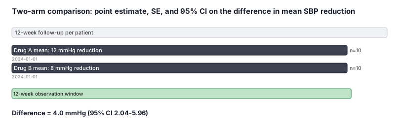
Consider a two-arm study comparing antihypertensive regimens in a claims-based cohort: 10 patients per arm, observed mean SBP reductions of 12.0 mmHg (Arm A) and 8.0 mmHg (Arm B). The analysis returns: mean difference = 4.0 mmHg, SE = 1.0, 95% CI [2.04, 5.96], z = 4.0, p < 0.001.

(1) Formal statistical interpretation. The point estimate of 4.0 mmHg is the observed difference in mean SBP reduction. The 95% CI [2.04, 5.96] is produced by a procedure that, if the study were repeated under identical conditions many times, would contain the true mean difference in approximately 95% of those replications; values of the true difference between 2.04 and 5.96 mmHg are compatible with the observed data at the 5% significance level. The p-value < 0.001 is the probability — under the null hypothesis that the true difference is exactly zero — of observing a difference at least as large as 4.0 mmHg in absolute value; it is not the probability that the null hypothesis is true.

(2) Practical interpretation for a decision-maker. Arm A reduced systolic blood pressure by roughly 4 more millimeters of mercury than Arm B, and the entire plausible range (2.0–6.0 mmHg) falls on the side favoring Arm A. Whether a 4 mmHg difference crosses the threshold of clinical importance depends on each patient's baseline risk, comorbidities, and tolerability — statistical significance alone does not establish that the difference is large enough to change treatment decisions.

Worked example

Scenario

A hospital quality team compares systolic blood pressure (SBP, in mmHg) reductions over 12 weeks for two antihypertensive drugs — Drug A (n = 10 patients) and Drug B (n = 10 patients). Drug A produces a mean reduction of 12 mmHg; Drug B produces a mean reduction of 8 mmHg. In both groups the variance of individual reductions is 5 mmHg². The team wants the point estimate of the difference, the standard error, a 95% confidence interval, and a test statistic to decide whether the difference is statistically significant.

Dataset

Summary statistics for a two-group blood-pressure reduction study (10 patients per arm).

Steps

• Point estimate: difference in mean reductions = 12.0 - 8.0 = 4.0 mmHg (Drug A reduces SBP by 4 mmHg more than Drug B on average).

• Standard error of the difference: SE = sqrt(variance_A/n_A + variance_B/n_B) = sqrt(5.0/10 + 5.0/10) = sqrt(0.5 + 0.5) = sqrt(1.0) = 1.0 mmHg. Note that this SE is about the estimate (the mean difference), not about individual patients — it tells us how much the 4.0 estimate would bounce if we ran the study again.

• 95% confidence interval: multiply the SE by the critical value 1.96 to get the margin. Margin = 1.96 * 1.0 = 1.96 mmHg. Lower bound = 4.0 - 1.96 = 2.04 mmHg; upper bound = 4.0 + 1.96 = 5.96 mmHg. Interpretation: the data are compatible with a true Drug A advantage of anywhere from about 2 to 6 mmHg — zero is not inside the interval.

• Test statistic: z = (estimate - null_value) / SE = (4.0 - 0) / 1.0 = 4.0 / 1.0 = 4.0. A z of 4.0 is far into the tail of the standard normal; the two-sided p-value is < 0.001.

• Clinical interpretation: the 4 mmHg difference is statistically significant (p < 0.001), but whether it is clinically meaningful depends on context — a 4 mmHg difference in a high-risk population may matter; in a low-risk one it may not. With only 10 patients per arm the CI spans 4 mmHg (2.04 to 5.96), which is moderately wide. In a claims database with 50,000 patients per arm, the CI might narrow to 3.8 to 4.2 mmHg — still significant but the same clinical question applies.

Result

Point estimate = 4.0 mmHg; SE = 1.0 mmHg; 95% CI = [2.04, 5.96] mmHg; z = 4.0; p < 0.001. The interval excludes zero, so the result is statistically significant at alpha = 0.05. The effect size (4 mmHg) and CI width (about 4 mmHg) together characterise the finding — the p-value alone does not.

Timeline Spec

Title

Two-arm comparison: point estimate, SE, and 95% CI on the difference in mean SBP reduction

Window

Start

2024-01-01

End

2024-12-31

Label

12-week follow-up per patient

Events

• Label

  Drug A mean: 12 mmHg reduction

  Start

  2024-01-01

  Length Days

  84

  Quantity

  n=10

• Label

  Drug B mean: 8 mmHg reduction

  Start

  2024-01-01

  Length Days

  84

  Quantity

  n=10

Spans

• Kind

  covered

  Start

  2024-01-01

  End

  2024-03-25

  Label

  12-week observation window

Result

Label

Difference = 4.0 mmHg (95% CI 2.04-5.96)

Value

4.0

Runnable example

import numpy as np
from scipy import stats

# --- From summary statistics (known n, mean, variance) ---
n_a, n_b = 10, 10
mean_a, mean_b = 12.0, 8.0
var_a, var_b = 5.0, 5.0     # variance of individual observations (SD^2), NOT SE^2

diff = mean_a - mean_b                          # point estimate of mean difference
se   = np.sqrt(var_a / n_a + var_b / n_b)       # SE of the difference: sqrt(s²/n + s²/n)
# Note: se != sqrt(var_a) or sqrt(var_b) — SD of the raw data is sqrt(var), SE is SD/sqrt(n)

z    = diff / se                                # z-statistic (large n; use t for small n)
ci_lo = diff - 1.96 * se                        # 95% CI lower bound
ci_hi = diff + 1.96 * se                        # 95% CI upper bound
p_val = 2 * (1 - stats.norm.cdf(abs(z)))        # two-sided p-value

print(f"Point estimate : {diff:.2f} mmHg")
print(f"SD of raw data : {np.sqrt(var_a):.3f} mmHg  (variability between individual patients)")
print(f"SE of estimate : {se:.3f} mmHg  (variability of the mean difference across repeated studies)")
print(f"95% CI         : [{ci_lo:.2f}, {ci_hi:.2f}] mmHg")
print(f"z-statistic    : {z:.2f}")
print(f"p-value        : {p_val:.4f}")

# --- From individual-level data (Welch's t-test, recommended when variances may differ) ---
rng = np.random.default_rng(42)
group_a = rng.normal(loc=mean_a, scale=np.sqrt(var_a), size=n_a)
group_b = rng.normal(loc=mean_b, scale=np.sqrt(var_b), size=n_b)
t_stat, p_ttest = stats.ttest_ind(group_a, group_b, equal_var=False)  # Welch's t-test
ci_ttest = stats.t.interval(0.95, df=len(group_a)+len(group_b)-2,
                            loc=group_a.mean()-group_b.mean(),
                            scale=stats.sem(group_a-group_b))
print(f"\nWelch t-test on simulated data: t={t_stat:.2f}, p={p_ttest:.4f}")
print(f"t-test 95% CI: [{ci_ttest[0]:.2f}, {ci_ttest[1]:.2f}]")

# --- From summary statistics ---
n_a <- 10L; n_b <- 10L
mean_a <- 12.0; mean_b <- 8.0
var_a  <- 5.0;  var_b  <- 5.0   # variance of raw observations (SD^2), NOT the SE

diff   <- mean_a - mean_b                      # point estimate
se_raw <- sqrt(var_a / n_a + var_b / n_b)      # SE of mean difference: sqrt(s^2/n + s^2/n)
# SD of raw data vs SE of estimate:
cat("SD of individual observations:", sqrt(var_a), "mmHg\n")
cat("SE of mean-difference estimate:", se_raw, "mmHg  (shrinks with n; SD does not)\n")

z      <- diff / se_raw
ci_lo  <- diff - 1.96 * se_raw
ci_hi  <- diff + 1.96 * se_raw
p_z    <- 2 * pnorm(-abs(z))

cat(sprintf("Point estimate : %.2f mmHg\n", diff))
cat(sprintf("SE             : %.3f mmHg\n", se_raw))
cat(sprintf("95%% CI         : [%.2f, %.2f] mmHg\n", ci_lo, ci_hi))
cat(sprintf("z-statistic    : %.2f\n", z))
cat(sprintf("p-value (z)    : %.4f\n\n", p_z))

# --- From individual-level data using base R t.test ---
set.seed(42)
group_a <- rnorm(n_a, mean = mean_a, sd = sqrt(var_a))
group_b <- rnorm(n_b, mean = mean_b, sd = sqrt(var_b))
tt      <- t.test(group_a, group_b, var.equal = FALSE)   # Welch's t-test
cat("t.test result:\n"); print(tt)

# --- Large-database demonstration: the 'significant but tiny' RWE trap ---
n_large  <- 500000L                     # half a million patients per arm (realistic claims n)
diff_tiny <- 0.05                       # 0.05 mmHg true difference — clinically negligible
se_large  <- sqrt(var_a / n_large + var_b / n_large)
z_large   <- diff_tiny / se_large
p_large   <- 2 * pnorm(-abs(z_large))
ci_large  <- c(diff_tiny - 1.96 * se_large, diff_tiny + 1.96 * se_large)
cat(sprintf("\n[Large-n demo] Diff = %.3f mmHg, SE = %.5f, z = %.1f, p = %.2e\n",
            diff_tiny, se_large, z_large, p_large))
cat(sprintf("95%% CI = [%.4f, %.4f] mmHg  -> significant but trivially small\n",
            ci_large[1], ci_large[2]))
cat("Lesson: in claims databases p < 0.05 is nearly automatic; report effect size + CI.\n")