Value of Information Analysis (EVPI, EVPPI, EVSI)

In plain language

Value of information analysis puts a dollar figure on what it would be worth to settle the remaining uncertainty in a cost-effectiveness decision before locking it in. Starting from the thousands of what-if model runs already produced for the analysis, it asks how often the apparently best treatment turns out to be the wrong pick and how much those mistakes cost. That ceiling (EVPI) is the most any future research on the question could ever be worth; the follow-on measures split it by which uncertain input drives it (EVPPI) and by the specific study you could actually run (EVSI), so an evidence budget goes to the study that buys the most decision certainty per dollar spent.

A probabilistic sensitivity analysis (PSA) ends with a distribution of outcomes, but the decision-maker still has to pick one strategy. Under current evidence the rational choice is the strategy with the highest expected net monetary benefit (NMB) — yet in some fraction of the PSA draws that choice is wrong, and each wrong draw carries a quantifiable opportunity loss (the NMB gap to that draw's true winner). Value of information (VOI) analysis is the formalization of that observation: the expected opportunity loss of deciding today is the expected value of removing the uncertainty. EVPI = E_theta[max_d NMB(d, theta)] - max_d E_theta[NMB(d, theta)]: average the per-draw best NMB, subtract the NMB of the strategy that is best on average. It is computed directly from the PSA matrix in two lines and is the upper bound on the value of any conceivable further research on this decision. The ISPOR VOI Good Practices Task Force (Fenwick et al. 2020; Rothery et al. 2020) frames the whole ladder: EVPI (all parameters, perfect information), EVPPI (perfect information on a parameter subset), EVSI (imperfect information from a specific finite study), and ENBS = population EVSI minus the study's cost — the quantity that actually decides whether to commission the study.

Estimation is where the craft lives

EVPI is nonparametric and free once the PSA exists. EVPPI naively requires a two-level nested Monte Carlo (an inner PSA for every outer draw of the parameter of interest) that is computationally brutal; the field-standard shortcut is the Strong–Oakley–Brennan regression estimator: regress each strategy's NMB on the parameter(s) of interest across the single existing PSA sample — a GAM/spline for 1–4 parameters, Gaussian-process regression for more — and the fitted values estimate E[NMB_d | theta]; EVPPI is then the mean of the per-draw fitted maxima minus the max of the column means. EVSI extends the same trick (Strong et al. 2015): for each PSA draw, simulate the summary statistic the proposed study would report (given its sample size, allocation, follow-up, and expected error), then regress NMB on that simulated statistic — the fitted values estimate the posterior-expected NMB after seeing the data. Population scaling multiplies per-patient VOI by the effective population: incident (plus prevalent, where the decision reaches them) patients per year x the decision-relevance horizon, with each future year's cohort discounted at the jurisdiction's rate. The horizon — how long the decision will stand before the technology landscape changes — is the most influential and least evidence-based input in the chain; report population VOI across 5/10/15-year horizons.

Pros, cons, and trade-offs

(specific and comparative). - vs probabilistic-sensitivity-analysis-hea-rwe (the substrate): PSA describes decision uncertainty (CEAC, scatter); VOI prices it and attaches a decision rule. A CEAC alone misleads in both directions: P(cost-effective) = 0.55 can carry trivial EVPI (the strategies are near-ties, being wrong costs little) or enormous EVPI (high stakes per patient, huge population). VOI is the only output that says whether the residual uncertainty matters. Cost: VOI inherits every distributional choice in the PSA — overdispersed or made-up priors inflate EVPI mechanically. - vs scenario-deterministic-sensitivity-analysis-hea-rwe (tornado/scenario): a tornado diagram ranks parameters by how far they swing the ICER; EVPPI ranks them by whether their uncertainty can flip the decision. A parameter can dominate the tornado yet have EVPPI near zero because no plausible value changes the adoption choice — and a modest parameter can carry most of the EVPPI because it sits exactly where strategies cross. For prioritizing research spend, EVPPI is the correct ranking; the tornado is a model-understanding tool. - vs heuristic research prioritization ("fund the biggest evidence gap"): VOI forces the gap to be valued against the population affected, the stakes per patient, and the cost and feasibility of the study that would close it. The price is machinery: a credible PSA, defensible effective-population assumptions, and for EVSI an explicit model of the future study's data-generating process — including, for RWE designs, its bias. Naive EVSI assumes the new data are an unbiased sample; an observational study with residual confounding delivers less (sometimes negative) value than its sample size suggests, so EVSI for RWE studies should model bias explicitly or be read as an upper bound.

When to use

Deciding whether a proposed RWE investment — a registry, a linked claims–EHR effectiveness study, a chart review to pin down utilities, a pragmatic trial — is worth its cost, and at what sample size (maximize ENBS, not power); prioritizing which parameter to spend an evidence budget on (EVPPI on relative effectiveness vs long-term survival extrapolation vs costs vs utilities points the money differently); HTA submissions and re-assessments, where coverage-with-evidence-development and managed-entry agreements are, operationally, decisions that the EVSI of further data collection exceeds its cost; research funders triaging portfolios across disease areas on population EVPI.

When NOT to use — and when it is actively misleading

- When structural uncertainty dominates. VOI computed from a PSA prices only parameter uncertainty. If the real doubt is the model structure (extrapolation functional form, comparator relevance, surrogate-to-final-outcome linkage), EVPI from the PSA understates the value of research — possibly by orders of magnitude. Parameterize structural choices into the PSA (model averaging) or do not present EVPI as "the" value of further research. - When the decision is not actually sensitive. If one strategy wins in ~100% of draws, EVPI is ~0 and the analysis is a one-line sanity check — do not build an EVSI machine to confirm a foregone conclusion. - When the PSA priors are not evidence-based. VOI is a precise function of the input distributions; arbitrary +/-20% uniforms produce arbitrary EVPI with impressive decimal places. Garbage in, confidently priced garbage out. - When the proposed study would be biased and the EVSI ignores it. EVSI that models an RWE study as unbiased sampling overstates its value; with material unmeasured confounding the study can even leave the decision-maker worse off (confidently wrong). Encode the design's expected bias and added variance, or present EVSI as an optimistic bound. - When delay costs are material and unmodeled. Patients are treated under current information while the study runs; an adopt-and-research vs delay-and-research framing changes ENBS and is a decision in itself.

Where the parameters come from (RWE operational depth)

In practice the PSA that feeds VOI is parameterized from real-world sources, and EVPPI tells you which source to go back to: cost and resource-use parameters typically come from claims (PPPM/PPPY costing studies); utilities and short-term effectiveness proxies from EHR or trial mapping; long-term survival, progression, and natural history — chronically the highest-EVPPI block in oncology and rare disease — from registries; and the proposed EVSI study is itself usually a linked-data design whose achievable precision and bias must be modeled honestly. VOI is therefore the budget-allocation layer that sits on top of the catalog's costing, utility, and survival-extrapolation machinery and decides which of them gets funded next.

Interpreting the output

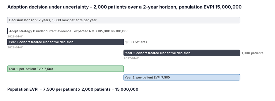
Consider the worked example: per-patient EVPI = 7,500 and population EVPI = 15,000,000 (2,000 patients over a 2-year decision horizon at a willingness-to-pay of 50,000 per QALY).

Formal interpretation: EVPI of 7,500 per patient is the expected cost of making a decision under current uncertainty — equivalently, the maximum worth paying per patient for any research that would resolve all uncertainty before the adoption decision is made. It is computed as the expected net monetary benefit under perfect information (112,500) minus the expected NMB of the best current decision (adopting B at 105,000). The population EVPI of 15,000,000 is that per-patient figure scaled by the number of patients who will be affected while the evidence gap persists. EVPI is strictly a function of the model's own probabilistic characterization of uncertainty — it measures how much the decision could improve if every uncertain parameter were resolved, not the value of any specific study design. EVPPI then partitions this ceiling across parameter groups to identify which inputs drive the most decision risk.

Practical interpretation: A population EVPI of 15,000,000 sets the ceiling for any research program targeting this decision: no single study or combination of studies is worth funding if its net cost exceeds that figure. Because the adoption decision was essentially a coin flip (probability 0.50 that B is optimal), substantial additional evidence is warranted before a final coverage determination. EVSI for a specific proposed RWE study — for example, a two-year comparative cohort in claims — will be lower than EVPI by the residual uncertainty the study cannot resolve and by any bias or variance the study design introduces. If the proposed study is expected to have material unmeasured confounding, model that expected bias explicitly; an optimistic EVSI that ignores study limitations will overstate the study's value.

Worked example

Scenario

A payer must choose between standard care (strategy A) and a new drug (strategy B) at a willingness-to-pay of 50,000 per QALY. To make every number checkable by hand, the modeling team's probabilistic sensitivity analysis is boiled down to just four equally likely simulations; standard care's cost and QALYs are well established, so they are the same in every draw, while the new drug's QALY gain is uncertain. We want the probability the adoption choice is wrong, the per-patient EVPI, and the population EVPI for 1,000 new patients per year over a 2-year decision horizon.

Dataset

Four equally likely PSA simulations - cost, QALYs, and net monetary benefit (NMB = 50,000 x QALYs - cost) for each strategy.

Steps

• Convert each strategy's cost and QALYs into net monetary benefit at the 50,000 threshold. For simulation 1, strategy B has NMB = 50,000 × 3.0 - 30,000 = 150,000 - 30,000 = 120,000, and strategy A has NMB = 50,000 × 2.4 - 20,000 = 100,000 in every simulation.

• Decide under current evidence using average NMB. Strategy A averages 100,000; strategy B averages (120,000 + 90,000 + 130,000 + 80,000) / 4 = 105,000. B wins on average, so today's decision is adopt B.

• Measure the decision uncertainty. B actually beats A only in simulations 1 and 3, so the probability that B is the right choice is 2/4 = 0.50 - the adoption decision is a coin flip.

• With perfect information you would pick each simulation's winner. The per-simulation best NMBs are 120,000; 100,000; 130,000; 100,000, so expected NMB with perfect information = (120,000 + 100,000 + 130,000 + 100,000) / 4 = 112,500.

• Per-patient EVPI = expected NMB with perfect information minus expected NMB of today's choice = 112,500 - 105,000 = 7,500. Equivalently it is the average opportunity loss of adopting B, since B loses by 10,000 in simulation 2 and by 20,000 in simulation 4, giving (0 + 10,000 + 0 + 20,000) / 4 = 7,500.

• Scale to the population the decision governs. With 1,000 new patients per year and a 2-year decision horizon, the affected population = 1,000 × 2 = 2,000 patients (discounting of the second-year cohort is omitted here for clarity; apply the jurisdiction's 3 percent rate in practice). Population EVPI = 7,500 × 2,000 = 15,000,000.

Result

Adopt B today (expected NMB 105,000 vs 100,000), but the choice is right in only 2/4 = 0.50 of simulations. Per-patient EVPI = 112,500 - 105,000 = 7,500, and population EVPI = 7,500 × 2,000 = 15,000,000 - so no research program costing more than 15 million can be worth funding on this decision, and EVPPI/EVSI then apportion that ceiling across the specific uncertain inputs and the specific RWE studies that could shrink them.

Timeline Spec

Title

Adoption decision under uncertainty - 2,000 patients over a 2-year horizon, population EVPI 15,000,000

Window

Start

2026-01-01

End

2027-12-31

Label

Decision horizon: 2 years, 1,000 new patients per year

Events

• Label

  Adopt strategy B under current evidence

  Start

  2026-01-01

  Length Days

  1

  Quantity

  expected NMB 105,000 vs 100,000

• Label

  Year 1 cohort treated under the decision

  Start

  2026-01-01

  Length Days

  365

  Quantity

  1,000 patients

• Label

  Year 2 cohort treated under the decision

  Start

  2027-01-01

  Length Days

  365

  Quantity

  1,000 patients

Spans

• Kind

  exposed

  Start

  2026-01-01

  End

  2026-12-31

  Label

  Year 1: per-patient EVPI 7,500

• Kind

  followup

  Start

  2027-01-01

  End

  2027-12-31

  Label

  Year 2: per-patient EVPI 7,500

Result

Label

Population EVPI = 7,500 per patient x 2,000 patients = 15,000,000

Value

15000000

Runnable example

import numpy as np

def evpi(nmb: np.ndarray) -> float:
    """nmb: (n_sims, n_strategies) net monetary benefit matrix from the PSA."""
    enb_current = nmb.mean(axis=0).max()   # best strategy on expected NMB (decide today)
    enb_perfect = nmb.max(axis=1).mean()   # per-draw winner, then average (perfect info)
    return float(enb_perfect - enb_current)

def evppi_regression(nmb: np.ndarray, theta: np.ndarray, degree: int = 3) -> float:
    """Strong-Oakley-Brennan: regress each strategy's NMB on the parameter(s) of
    interest; fitted values estimate E[NMB_d | theta]. Polynomial here for zero
    dependencies - use a GAM (1-4 params) or GP regression (more) in production."""
    theta = np.asarray(theta, dtype=float)
    fitted = np.column_stack([
        np.polyval(np.polyfit(theta, nmb[:, d], degree), theta)
        for d in range(nmb.shape[1])
    ])
    return float(fitted.max(axis=1).mean() - nmb.mean(axis=0).max())

def evsi_regression(nmb: np.ndarray, future_summary: np.ndarray, degree: int = 3) -> float:
    """EVSI (Strong 2015): same estimator, but the regressor is the summary statistic
    the PROPOSED study would report, simulated once per PSA draw from its design."""
    return evppi_regression(nmb, future_summary, degree=degree)

def effective_population(incidence_per_year: float, horizon_years: int,
                         discount_rate: float = 0.03) -> float:
    """Discounted number of patients the decision affects over its relevance horizon."""
    return sum(incidence_per_year / (1.0 + discount_rate) ** t for t in range(horizon_years))

# --- demo: two-strategy PSA where the relative risk carries the decision value ---
rng = np.random.default_rng(2026)
n_sims, lam = 5000, 50_000
rr       = rng.normal(0.75, 0.10, n_sims)      # uncertain treatment effect
qaly_a   = rng.normal(2.4, 0.20, n_sims)
cost_a   = rng.normal(20_000, 2_000, n_sims)
inc_cost = rng.gamma(25.0, 400.0, n_sims)      # incremental cost of B
nmb = np.column_stack([
    lam * qaly_a - cost_a,                                        # A: standard care
    lam * (qaly_a + (1.0 - rr) * 0.8) - (cost_a + inc_cost),      # B: new drug
])

per_person = evpi(nmb)
rr_hat = rng.normal(rr, 0.07)   # proposed RWE study reports rr with SE 0.07
print(f"P(B optimal)            : {(nmb[:, 1] > nmb[:, 0]).mean():.3f}")
print(f"EVPI per person         : {per_person:,.0f}")
print(f"EVPPI(rr)               : {evppi_regression(nmb, rr):,.0f}")
print(f"EVPPI(incremental cost) : {evppi_regression(nmb, inc_cost):,.0f}")
print(f"EVSI(rr study, SE 0.07) : {evsi_regression(nmb, rr_hat):,.0f}")
print(f"Population EVPI (10y)   : {per_person * effective_population(1_000, 10):,.0f}")

library(mgcv)

evpi <- function(nmb) {
  # nmb: n_sims x n_strategies NMB matrix from the PSA
  mean(apply(nmb, 1, max)) - max(colMeans(nmb))
}

evppi_gam <- function(nmb, theta) {
  # Strong-Oakley-Brennan: fitted values of gam(NMB_d ~ s(theta)) estimate E[NMB_d | theta]
  fitted_nmb <- sapply(seq_len(ncol(nmb)), function(d)
    fitted(gam(nmb[, d] ~ s(theta))))
  mean(apply(fitted_nmb, 1, max)) - max(colMeans(nmb))
}

effective_population <- function(incidence_per_year, horizon_years, discount_rate = 0.03) {
  sum(incidence_per_year / (1 + discount_rate)^(0:(horizon_years - 1)))
}

# --- demo: two-strategy PSA where the relative risk carries the decision value ---
set.seed(2026)
n_sims <- 5000; lam <- 50000
rr       <- rnorm(n_sims, 0.75, 0.10)        # uncertain treatment effect
qaly_a   <- rnorm(n_sims, 2.4, 0.20)
cost_a   <- rnorm(n_sims, 20000, 2000)
inc_cost <- rgamma(n_sims, shape = 25, scale = 400)
nmb <- cbind(A = lam * qaly_a - cost_a,
             B = lam * (qaly_a + (1 - rr) * 0.8) - (cost_a + inc_cost))

per_person <- evpi(nmb)
rr_hat <- rnorm(n_sims, mean = rr, sd = 0.07)  # proposed RWE study estimate of rr
cat(sprintf("P(B optimal)            : %.3f\n", mean(nmb[, "B"] > nmb[, "A"])))
cat(sprintf("EVPI per person         : %s\n", format(round(per_person), big.mark = ",")))
cat(sprintf("EVPPI(rr)               : %s\n", format(round(evppi_gam(nmb, rr)), big.mark = ",")))
cat(sprintf("EVPPI(incremental cost) : %s\n", format(round(evppi_gam(nmb, inc_cost)), big.mark = ",")))
cat(sprintf("EVSI(rr study, SE 0.07) : %s\n", format(round(evppi_gam(nmb, rr_hat)), big.mark = ",")))
cat(sprintf("Population EVPI (10y)   : %s\n",
            format(round(per_person * effective_population(1000, 10)), big.mark = ",")))