Confounding control · Implementation

Love Plot (Standardized Mean Differences)

Covariate balance diagnostic: the absolute standardized mean difference for each confounder, before and after matching or weighting, against a 0.10 threshold.

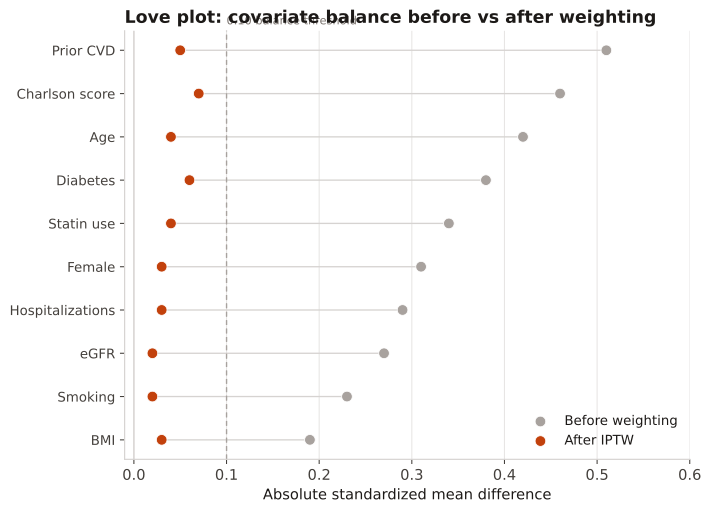
Download SVG Open code and full worked example

When to use it

To show that a propensity-score adjustment achieved balance. The SMD is preferred over a p-value because it is independent of sample size; |SMD|<0.10 is the conventional balance target.

How to read it

Each covariate has a 'before' and 'after' dot; adjustment should pull the after-dots left of 0.10. Residual imbalance above 0.10 flags a covariate to add to the PS model or the outcome model.

Worked example

Ten baseline covariates compared between treated and control before and after IPTW. The SMD is (x̄_treated − x̄_control) divided by the pooled standard deviation; the absolute value is plotted.

Prior CVD before |SMD|=0.51 → after 0.05; Charlson before 0.46 → after 0.07; Age before 0.42 → after 0.04; …

Result: Before weighting, 10/10 covariates exceed 0.10 (max 0.51 for prior CVD); after IPTW all 10 fall below 0.10 (max 0.07), so the weighted pseudo-population is balanced and the outcome model can proceed.

Produced by

Propensity-score methods (matching, IPTW)Baseline characteristics & covariate balance High-dimensional propensity score (hdPS)

Reference: Gatto NM, Wang SV, Murk W, et al. Visualizations throughout pharmacoepidemiology study planning, implementation, and reporting. Pharmacoepidemiol Drug Saf. 2022;31(11):1140-1152.