Case-Case-Time-Control Design

In plain language

The case-case-time-control design answers the question: does taking a drug in the days just before an acute event actually raise the risk, after accounting for the fact that more people are using the drug over time? For each person who had the event, it compares whether they were on the drug in the 30 days right before the injury to whether they were on it in an earlier 30-day window from the same person, so their stable background characteristics cancel out. It then corrects a hidden problem with that simple within-person comparison: if drug use in the whole population has been rising over calendar time, the window closest to the event will always look more exposed just because of the calendar, not because of a real risk. To fix that, the design borrows a second group, people who had the same event later, and runs the identical within-person comparison on them to measure how much of the difference was just the calendar trend; dividing the two results gives the trend-corrected estimate.

The case-case-time-control (CCTC) design is a self-controlled, case-only design for transient (acute, short-induction) drug effects. It corrects the one bias the case-crossover cannot fix on its own: a secular exposure-time trend. The estimator is a ratio of two conditional odds ratios. First, run an ordinary case-crossover in the cases: within each case, compare exposure in a hazard window just before the event to exposure in one or more earlier reference windows. This self-matched odds ratio (OR_case) cancels every time-invariant confounder — measured or not — because each person is their own control. But OR_case is contaminated if drug use is trending over calendar time (uptake of a new agent, decline after a warning), because the hazard window is, by construction, later than the reference window. CCTC estimates that trend from a comparator group of future cases — people who experience the same outcome but later — by running the identical self-matched comparison shifted onto their (pre-event) calendar period, yielding OR_futurecase. The causal estimate is OR_CCTC = OR_case / OR_futurecase, a ratio of conditional ORs typically obtained as the exposure × group interaction in a single conditional logistic model. Design and estimator are inseparable here: building the windows without the ratio is not the method.

Conceptual lineage (the spine)

Maclure 1991 (case-crossover) introduced within-person comparison of hazard vs reference windows, removing fixed confounding but assuming no exposure-time trend. Suissa 1995 (case-time-control) added a concurrent control group — non-cases — to estimate and divide out that trend. The fatal weakness of case-time-control is that drug-use trends in non-cases need not equal trends in cases: if the disease itself drives prescribing (confounding by indication has a temporal analogue), non-cases mis-measure the cases' counterfactual trend. Wang 2011 (CCTC) replaced the non-case time controls with future cases, who share the cases' indication, severity trajectory, and prescribing dynamics, so their pre-event exposure trend is a far better proxy for what the current cases' trend would have been absent the event. CCTC is therefore best read as case-time-control with a sharper choice of time control.

Pros, cons, and trade-offs

- vs case-crossover: CCTC removes the exposure-time-trend bias that case-crossover silently carries whenever drug use drifts over calendar time (almost always true for newer drugs, post-warning drugs, or anything seasonal). Cost: it needs a future-case sample, roughly doubles data requirements, and inflates variance (you are dividing two noisy ORs). Prefer case-crossover only when you can defend a flat exposure trend (e.g., a long-established drug at steady-state use); otherwise prefer CCTC. - vs case-time-control (non-case controls): CCTC's future cases share indication and channeling with the cases, so the trend correction is less biased than Suissa's non-case correction whenever the outcome influences exposure trends. Cost: future cases are scarcer than non-cases (you must wait for them to accrue) and require enough post-index follow-up to identify them. Prefer CCTC in pharmacoepidemiology, where indication-driven prescribing is the norm. - vs self-controlled case series (SCCS): SCCS models the full observation time and is more efficient for recurrent or well-defined transient exposures, but it requires that the event not censor or alter future exposure (the event-dependent-exposure assumption) and that exposures be modeled as time-varying covariates. CCTC makes no parametric rate model and tolerates event-dependent exposure better, but estimates only a transient (window-contrast) effect. Prefer SCCS for vaccine-style point exposures with clean rate models; prefer CCTC for chronically-trending drug exposures where event-dependent exposure and secular trend coexist. - vs cohort / active-comparator new-user designs: CCTC needs no measured confounders and no external comparator cohort, a decisive advantage when key confounders are unrecorded. Cost: it cannot estimate effects of time-invariant exposures (a within-person design has no variation in them), gives only relative (not absolute) effects, and answers a transient- effect question, not a cumulative or long-latency one. Prefer a cohort/ACNU design for chronic cumulative effects or when absolute risk is required.

When to use

Acute outcomes with a plausible transient drug trigger (induction period of days to weeks): e.g., fracture or fall after a sedating drug, GI bleed after an NSAID, MI after a COX-2 inhibitor, hip fracture after a benzodiazepine. Settings where the dominant confounders (frailty, baseline disease severity, genetics) are time-invariant and unmeasured, so a within-person design is attractive — and where drug use is clearly trending over calendar time, so a plain case-crossover would be biased. CCTC is well suited to administrative claims, where dispensing dates and a large pool of future cases are both available.

When NOT to use — and when it is actively misleading

- The exposure trend differs between current and future cases. This is the load-bearing assumption: future cases' pre-event exposure trend must equal the current cases' counterfactual trend. It breaks under rapid drug launch/uptake or post-warning withdrawal (the trend is changing too fast for a fixed future offset to track), mid-window guideline changes, formulary switches, or shifting diagnostic criteria that redefine who becomes a case over calendar time. If the trend is non-linear or regime-changing across the study period, OR_CCTC is not interpretable. - The effect is cumulative or long-latency, not transient. A within-person hazard-vs-reference contrast cannot capture effects that build over months/years; the reference window would itself be "exposed" in causal terms. Use a cohort design. - The exposure is stable within person (time-invariant or near-constant chronic use): there is no within-person discordance to estimate from, and the OR is undefined or unstable. Self-controlled designs need exposure switching. - Event-dependent exposure with strong feedback. If the event itself sharply changes exposure (hospitalization stops outpatient fills), the reference windows must be chosen before the event and any post-event period excluded; naive bidirectional windows reintroduce bias. - Too few future cases or too-short follow-up. Sparse future cases make OR_futurecase unstable; dividing by a noisy denominator can produce wild point estimates and intervals. Pre-specify a minimum future-case sample.

Data-source operational depth

- Claims (FFS): The natural substrate. Exposure on a given day is reconstructed from `fill_date` + `days_supply` (a person is "exposed" on day d if some fill covers d). The hazard window is the N days immediately before the event date; reference windows are equal-length windows further back (and, for future cases, windows before their later event). Failure modes: (1) Medicare Advantage / capitated person-time lacks fee-for-service pharmacy claims, so "unexposed" windows can be unobserved exposure — restrict to enrollees with full Part D (or commercial pharmacy benefit) covering all windows. (2) 90-day mail-order and stockpiling distort daily exposure status; cap or carry-over `days_supply` consistently in cases and future cases. (3) Reference and hazard windows must lie inside continuous enrollment, or window exposure is censored asymmetrically. - EHR: Exposure is the order/administration, not the dispensing; outpatient adherence is unknown, so transient triggering is mismeasured unless linked to fills. Visit-driven capture means windows with no encounter look "unexposed" spuriously. Outcome dates from notes/labs may lag the true event, blurring the hazard window — anchor on the most objective date available (e.g., admission date). - Registry: Adjudicated outcome timing is a strength (clean hazard-window anchoring); pharmacy exposure is usually weak and must be linked to claims for daily exposure reconstruction. - Linked claims–EHR: Ideal — EHR for precise event dating and indication, claims for complete day-level exposure — but reconcile order/fill/service dates before assigning windows; a date discrepancy of days can move a fill across the hazard/reference boundary and flip a discordant pair.

Worked claims example

Question: does initiating a sedating antipsychotic acutely trigger hip fracture in elderly nursing-home residents (Wang 2011's setting)? (1) Cases: residents with an incident hip-fracture admission; `event_date` = admission date; require continuous Part A/B/D enrollment with no MA-only person-time spanning all windows. (2) Windows: hazard window = days 1–30 before `event_date`; reference window = days 91–120 before `event_date` (equal 30-day length, separated by a washout to avoid carry-over). A person is "exposed" in a window if any antipsychotic fill (`fill_date` + `days_supply`) covers ≥1 day of it. (3) Case-crossover OR (OR_case): conditional logistic regression stratified on `person_id`, two rows per case (hazard vs reference), exposure as the predictor — say OR_case = 2.4. This still embeds the rising secular use of antipsychotics in this population. (4) Future cases: residents who fracture later in the data; apply the same day-30 hazard / day-91–120 reference windows anchored on their own later event, capturing the calendar-time exposure trend — say OR_futurecase = 1.6. (5) CCTC estimate: OR_CCTC = OR_case / OR_futurecase = 2.4 / 1.6 = 1.5, the trend-adjusted transient effect. Operationally this is one conditional logistic model on the pooled case + future-case rows with an exposure × group(current vs future) interaction; the interaction odds ratio is OR_CCTC, and its model-based CI propagates both ORs' uncertainty.

Worked example

Scenario

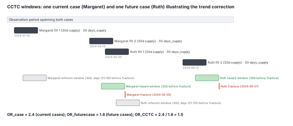
We want to know whether starting an antipsychotic pill acutely raises the risk of a hip fracture in elderly nursing-home residents. We use insurance claims, where pharmacy fills record the drug name, the fill date, and how many days that supply lasts. Two residents fractured their hip: Margaret fractured on 2024-05-30 (she is a current case), and Ruth fractured on 2024-09-27 (she is a future case, the same outcome but later in calendar time, used to measure the drug-use trend). We look at each woman's own prescription history to decide whether she was on an antipsychotic in her hazard window and in her referent window.

Dataset

Pharmacy fills for two residents in the claims data (simplified to one drug each)

Steps

• Define windows for Margaret (current case, event 2024-05-30): hazard window = 2024-04-30 to 2024-05-29 (30 days before the fracture); referent window = 2024-01-21 to 2024-02-19 (30 days ending 90 days before the hazard window starts, so days 121-150 before the event).

• Check Margaret's fills against her windows: her 2024-04-15 fill (30 days supply) covers through 2024-05-14, which overlaps the hazard window (Apr 30 - May 29), so she is EXPOSED in the hazard window. Her 2024-01-10 fill (30 days supply) covers through 2024-02-08, which overlaps the referent window (Jan 21 - Feb 19), so she is EXPOSED in the referent window. Margaret is concordant (exposed in both), so her pair contributes no discordance to the within-person comparison.

• Now define windows for Ruth (future case, event 2024-09-27): same rule, shifted to her own event date. Hazard window = 2024-08-28 to 2024-09-26; referent window = 2024-05-19 to 2024-06-17.

• Check Ruth's fills: her 2024-08-12 fill covers through 2024-09-10, overlapping her hazard window, so EXPOSED in hazard. Her 2024-05-05 fill covers through 2024-06-03, which overlaps her referent window (May 19 - Jun 17), so EXPOSED in referent. Ruth is also concordant in this simple two-person illustration.

• In a full study with many such pairs, the within-current-case comparison yields OR_case = 2.4 (the raw within-person odds ratio suggesting higher exposure near the fracture). The within-future-case comparison yields OR_futurecase = 1.6 (capturing the secular rise in antipsychotic use over calendar time that makes every later window look more exposed).

• The trend-adjusted estimate is OR_CCTC = OR_case divided by OR_futurecase = 2.4 / 1.6 = 1.5. This means after removing the calendar trend, being on an antipsychotic in the 30 days before a hip fracture is associated with 1.5 times the odds of fracture compared with an earlier period, not 2.4 times.

Result

OR_CCTC = 2.4 / 1.6 = 1.5. The raw within-person signal of 2.4 was inflated by rising antipsychotic use over calendar time; after the future-case trend correction the estimate drops to 1.5.

Timeline Spec

Title

CCTC windows: one current case (Margaret) and one future case (Ruth) illustrating the trend correction

Window

Start

2024-01-01

End

2024-10-15

Label

Observation period spanning both cases

Events

• Label

  Margaret fill 1 (30d supply)

  Start

  2024-01-10

  Length Days

  30

  Quantity

  30 days_supply

• Label

  Margaret fill 2 (30d supply)

  Start

  2024-04-15

  Length Days

  30

  Quantity

  30 days_supply

• Label

  Ruth fill 1 (30d supply)

  Start

  2024-05-05

  Length Days

  30

  Quantity

  30 days_supply

• Label

  Ruth fill 2 (30d supply)

  Start

  2024-08-12

  Length Days

  30

  Quantity

  30 days_supply

Spans

• Kind

  unexposed

  Start

  2024-01-21

  End

  2024-02-19

  Label

  Margaret referent window (30d, days 121-150 before fracture)

• Kind

  exposed

  Start

  2024-04-30

  End

  2024-05-29

  Label

  Margaret hazard window (30d before fracture)

• Kind

  gap

  Start

  2024-05-30

  End

  2024-05-30

  Label

  Margaret fracture (2024-05-30)

• Kind

  unexposed

  Start

  2024-05-19

  End

  2024-06-17

  Label

  Ruth referent window (30d, days 121-150 before fracture)

• Kind

  exposed

  Start

  2024-08-28

  End

  2024-09-26

  Label

  Ruth hazard window (30d before fracture)

• Kind

  gap

  Start

  2024-09-27

  End

  2024-09-27

  Label

  Ruth fracture (2024-09-27)

Result

Label

OR_case = 2.4 (current cases); OR_futurecase = 1.6 (future cases); OR_CCTC = 2.4 / 1.6 = 1.5

Value

1.5

Caption

Two residents share the same window structure anchored on their own event dates. Margaret is a current case (fracture May 30); Ruth is a future case (fracture Sep 27) used to estimate the calendar-time trend in antipsychotic use. Dividing the within-current-case odds ratio (2.4) by the within-future-case odds ratio (1.6) removes the trend and yields the corrected estimate of 1.5.

Alt Text

Horizontal timeline from January to October 2024 showing fill bars and shaded referent and hazard windows for Margaret (current case, fracture May 30) and Ruth (future case, fracture Sep 27), illustrating how the same window structure applied to a later case estimates the secular drug-use trend.

Runnable example

import pandas as pd
import numpy as np
import statsmodels.api as sm
from statsmodels.discrete.conditional_models import ConditionalLogit

HAZARD_DAYS = 30          # day 1..30 before the event
REF_GAP_DAYS = 90         # washout between hazard and reference window
REF_DAYS = 30             # reference window length (equal to hazard)

def _covered(rx_p, w_start, w_end):
    """True if any fill's [fill_date, fill_date+days_supply) covers >=1 day of [w_start, w_end]."""
    supply_end = rx_p["fill_date"] + pd.to_timedelta(rx_p["days_supply"], unit="D")
    return bool(((rx_p["fill_date"] <= w_end) & (supply_end > w_start)).any())

def _enrolled(enr_p, w_start, w_end):
    """True if a single non-MA enrollment span fully covers the window (so 'unexposed' is observed, not missing)."""
    ok = (enr_p["enroll_start"] <= w_start) & (enr_p["enroll_end"] >= w_end) & (~enr_p["ma_only"])
    return bool(ok.any())

def build_cctc_rows(events, rx, enroll):
    rows = []
    rx_by = dict(tuple(rx.groupby("person_id")))
    en_by = dict(tuple(enroll.groupby("person_id")))
    for _, ev in events.iterrows():
        pid, e0, grp = ev["person_id"], ev["event_date"], ev["group"]
        haz = (e0 - pd.Timedelta(days=HAZARD_DAYS), e0 - pd.Timedelta(days=1))
        ref_end = e0 - pd.Timedelta(days=HAZARD_DAYS + REF_GAP_DAYS)
        ref = (ref_end - pd.Timedelta(days=REF_DAYS - 1), ref_end)
        rx_p = rx_by.get(pid, rx.iloc[0:0])
        en_p = en_by.get(pid, enroll.iloc[0:0])
        # Both windows must be observable; otherwise the discordant pair is censored asymmetrically -> drop the case.
        if not (_enrolled(en_p, *haz) and _enrolled(en_p, *ref)):
            continue
        rows.append({"person_id": pid, "group": grp, "window": "hazard",
                     "exposed": int(_covered(rx_p, *haz))})
        rows.append({"person_id": pid, "group": grp, "window": "reference",
                     "exposed": int(_covered(rx_p, *ref))})
    return pd.DataFrame(rows)

def estimate_cctc(rows):
    d = rows.copy()
    d["hazard"] = (d["window"] == "hazard").astype(int)             # within-person time contrast
    d["future"] = (d["group"] == "future").astype(int)
    d["hazard_x_future"] = d["hazard"] * d["future"]                # interaction = trend correction
    # Conditional logistic, stratified on person; outcome = exposed in that window.
    X = d[["hazard", "hazard_x_future"]]
    model = ConditionalLogit(d["exposed"], X, groups=d["person_id"])
    res = model.fit(disp=False)
    # OR_case = exp(hazard); OR_futurecase = exp(hazard + hazard_x_future);
    # OR_CCTC = OR_case / OR_futurecase = exp(-hazard_x_future).
    beta_int = res.params["hazard_x_future"]
    or_cctc = float(np.exp(-beta_int))
    ci = np.exp(-res.conf_int().loc["hazard_x_future"][::-1])       # flip sign -> flip/relabel bounds
    return {"OR_case": float(np.exp(res.params["hazard"])),
            "OR_CCTC": or_cctc, "CI95": (float(ci[0]), float(ci[1]))}

library(data.table)
library(survival)

HAZARD_DAYS <- 30L; REF_GAP_DAYS <- 90L; REF_DAYS <- 30L

covered <- function(fd, ds, ws, we) any(fd <= we & (fd + ds) > ws)
enrolled <- function(es, ee, mao, ws, we) any(es <= ws & ee >= we & !mao)

build_cctc_rows <- function(events, rx, enroll) {
  setDT(events); setDT(rx); setDT(enroll)
  out <- list()
  for (i in seq_len(nrow(events))) {
    pid <- events$person_id[i]; e0 <- events$event_date[i]; grp <- events$group[i]
    haz_s <- e0 - HAZARD_DAYS;            haz_e <- e0 - 1L
    ref_e <- e0 - (HAZARD_DAYS + REF_GAP_DAYS); ref_s <- ref_e - (REF_DAYS - 1L)
    rp <- rx[person_id == pid]; ep <- enroll[person_id == pid]
    # Both windows must be observable, non-MA, or the discordant pair is censored asymmetrically -> drop.
    if (!(enrolled(ep$enroll_start, ep$enroll_end, ep$ma_only, haz_s, haz_e) &&
          enrolled(ep$enroll_start, ep$enroll_end, ep$ma_only, ref_s, ref_e))) next
    out[[length(out) + 1L]] <- data.table(
      person_id = pid, group = grp, window = c("hazard", "reference"),
      exposed = c(as.integer(covered(rp$fill_date, rp$days_supply, haz_s, haz_e)),
                  as.integer(covered(rp$fill_date, rp$days_supply, ref_s, ref_e))))
  }
  rbindlist(out)
}

estimate_cctc <- function(rows) {
  rows[, hazard := as.integer(window == "hazard")]   # within-person time contrast
  rows[, future := as.integer(group == "future")]
  # Conditional logistic stratified on person; exposed ~ hazard * future, strata(person).
  fit <- clogit(exposed ~ hazard + hazard:future + strata(person_id), data = rows)
  b_int <- coef(fit)["hazard:future"]
  ci <- exp(-rev(confint(fit)["hazard:future", ]))   # OR_CCTC = exp(-interaction)
  list(OR_case = unname(exp(coef(fit)["hazard"])),
       OR_CCTC = unname(exp(-b_int)),
       CI95 = unname(ci))
}