Case-Crossover Design
A self-controlled design in which each case serves as its own control, contrasting exposure during a hazard ("case") window immediately before an acute event with exposure during one or more earlier referent ("control") windows in the same person, to estimate the transient effect of an intermittent exposure on the risk of abrupt event onset.
On this page
A case-crossover study asks: was the patient more likely to be taking a short-acting drug in the days just before their emergency hospitalization than they were in calmer periods months earlier? Instead of comparing the patient to other people, the design compares the same person to themselves — the hazard window (a brief period right before the event) versus earlier referent windows when no event occurred. Because both windows come from the same person, anything that is stable about them — their chronic conditions, genetics, income, general frailty — automatically cancels out. The trade-off is that it only works when the exposure is intermittent (taken sometimes but not always) and the event is sudden and well-dated, like a hospitalization.
The case-crossover design studies whether a transient exposure triggers an abrupt event by comparing, within each case, the exposure status during a short window just before the event (the case/hazard window) with exposure during one or more referent/control windows in that same individual at an earlier time. There is no separate control group: each case is matched to itself. Analytically it is a matched case-control study where the matched sets are person-periods, so the natural estimator is conditional (stratum = person) logistic regression, and the estimand is the odds ratio for the transient effect of exposure on event onset within the hazard window (an approximation of the rate ratio under the usual rare-event/incidence-density logic of Mittleman, Maclure & Robins).
Core conceptual distinction — why self-controlled
Because both windows come from the same person, every time-invariant characteristic is matched out by design: genetics, sex, baseline comorbidity, frailty, socioeconomic status, chronic channeling, and any other stable confounder — measured or not — cancels in the within-person contrast. This is the design's unique selling point relative to cohort or conventional case-control designs, which must measure and adjust for those confounders. The price is that the design controls only time-invariant confounding; anything that varies within a person over the spacing between windows (acute illness, season, day of week, secular trends in exposure prevalence) is not controlled and can bias the estimate badly.
Estimand and assumptions
Under (i) a transient exposure with a well-defined effect (induction/hazard) period, (ii) a stable distribution of exposure over time within persons (the "no exposure-time trend" assumption), (iii) no carryover of effect from the case window into the referent windows (and vice versa), and (iv) the event not itself altering subsequent exposure, the conditional-logistic OR estimates the incidence rate ratio for the acute triggering effect. Violations of (ii) and (iii) are the dominant failure modes and motivate the case-time-control and case-case-time-control extensions below.
Pros, cons, and trade-offs
- vs cohort / new-user designs: Case-crossover needs no comparator cohort and is immune to all stable confounding, which is decisive when the suspected confounders are chronic and hard to measure in claims (frailty, lifestyle). Cost: it answers only the transient-trigger question, gives an OR not an absolute risk, has no information on chronic-exposure effects, and is vulnerable to within-person time trends that a cohort with an external comparator can absorb. Prefer for short-acting drugs and acute events where confounding-by-indication and unmeasured frailty would wreck a cohort.
- vs conventional / nested case-control: Removes between-person confounding entirely and needs no control selection, eliminating one source of selection bias. Cost: it cannot study non-time-varying exposures, is less efficient when exposure is rare or near-constant within persons, and shifts the threat from confounding to exposure-trend bias.
- vs self-controlled case series (SCCS): Both are self-controlled and remove time-invariant confounding. SCCS models the full observation time with a Poisson/conditional-Poisson model, handles recurrent events naturally, requires the event not to censor/curtail observation (or a modified SCCS), and is well suited to vaccine-safety risk-interval analyses. Case-crossover samples discrete referent windows, needs only the cases, and is simpler when the exposure is sharply intermittent and the event is acute and rare. Prefer SCCS for recurrent events or when modeling age/time effects explicitly; prefer case-crossover for a single acute event triggered by a sharply transient exposure.
- vs case-time-control / case-case-time-control: When background exposure prevalence is changing over calendar time (e.g., a drug's use is rising), the plain case-crossover OR is biased by that exposure-time trend. Case-time-control (Suissa 1995) adds a separate control group to estimate and subtract the trend; case-case-time-control (Wang, Schneeweiss) uses future cases as the control series to also absorb within-person trends from disease progression. These are the correct fixes, not heavier covariate adjustment.
When NOT to use — and when it is actively misleading or dangerous
- Chronic / continuous exposure. If exposure is essentially constant across the case and referent windows (a maintenance statin taken daily for years), there is no within-person contrast and the design is uninformative or biased toward the null. Use a cohort/new-user design instead.
- Exposure with a secular time trend. If the drug's prevalence is rising (or falling) over calendar time, exposure is systematically more (or less) likely in the more recent case window than in earlier referent windows for reasons unrelated to the event, producing a spurious OR. This is the canonical case-crossover failure and is exactly what case-time-control repairs. Bidirectional sampling (referent windows both before and after the event) partly mitigates it but assumes the event does not affect future exposure.
- Carryover / long or ill-defined effect window. If the effect persists across both windows, or the induction period is long relative to window spacing, exposure "bleeds" into the referent window and attenuates the contrast. Case-crossover demands a short, well-characterized hazard period.
- Event alters subsequent exposure (within-person reverse causation). If a prodrome of the event changes exposure (a patient with early symptoms stops or starts a drug), unidirectional (before-only) sampling is biased; bidirectional sampling is invalid because post-event exposure is affected by the event.
- Depletion of susceptibles / first-event-only chronic use. For drugs where susceptible patients have their event early in treatment, the within-person exposure-event association is distorted; SCCS or a new-user cohort is safer.
Operational sampling choices (these are design decisions, not nuisances)
Unidirectional sampling draws referent windows only before the event (mandatory when the event can affect future exposure or cause death); it is the more conservative default in pharmacoepidemiology. Bidirectional sampling draws referents both before and after the event and controls for within-person time trends, but is valid only when post-event exposure is unaffected by the event. The number and spacing of referent windows trade efficiency against the exposure-trend and carryover assumptions: more referent windows improve precision (Mittleman, Maclure & Robins show the relative efficiency gains) but widen the calendar span over which the no-trend assumption must hold. A further choice is the point-in-time approach (was the person exposed on the index day of each window?) vs the window/hazard-period approach (was there any exposure within a multi-day hazard period?); in claims the window approach with a `days_supply`-defined exposure interval is usually required because dispensing is bursty (Hallas et al. 2024).
Data-source operational depth
- Claims (FFS): Exposure is reconstructed from pharmacy fills — a person is "exposed" on a given day if a dispensing's `[fill_date, fill_date + days_supply)` interval covers that day (apply a grace period and stockpiling rule, and account for 90-day mail-order and free samples that distort `days_supply`). The event date is the index claim for the acute outcome. Require continuous medical + pharmacy enrollment spanning the entire span from the earliest referent window through the event so that absence of a fill is true non-exposure, not unobserved dispensing. Failure modes: Medicare Advantage and capitated person-time lack fee-for-service claims, so exposure in a referent window can be missing rather than absent — restrict to enrollees with the relevant medical + Part D / pharmacy benefit and exclude MA-only person-time across every window. Outpatient-only acute events may be miscoded or undated; prefer inpatient/ED principal-diagnosis events with a clean admission date as the anchor.
- EHR: Exposure is the order/administration, not the fill, and is visit-driven, so the referent windows are populated only when the patient interacts with the system — differential visit intensity around the event (more contact just before an MI) manufactures a spurious within-person exposure trend. Link to dispensing where possible and restrict to exposures routinely captured (e.g., inpatient MAR) rather than self-managed OTC drugs.
- Registry / linked: Registries give well-adjudicated, well-dated acute events (the ideal anchor) but rarely complete longitudinal exposure; link to claims for the fill history and to a death index, since unidirectional sampling is mandatory when the event is fatal (no post-event windows exist).
Worked claims example
Question: does short-term NSAID exposure trigger acute upper-GI bleeding among older adults in a Medicare FFS + Part D database?
- Cases: the first hospitalization with a principal ICD-10 diagnosis of acute upper-GI hemorrhage; the event date is the admission date.
- Enrollment: require continuous Parts A/B/D and exclude any MA-only person-time over the 6 months preceding the event so every window is FFS-observable.
- Exposure: a day is NSAID-exposed if any non-aspirin NSAID dispensing's `[fill_date, fill_date + days_supply + 3-day grace)` interval covers it.
- Hazard (case) window: the 7 days immediately before the event date.
- Referent (control) windows: four non-overlapping 7-day windows ending 30, 60, 90, and 120 days before the event (unidirectional, because the bleed and any hospitalization can alter subsequent drug use).
- Classify each window as exposed/unexposed by the rule in (3), creating one stratum per person with one case-window row and four referent-window rows.
- Fit conditional logistic regression stratified on `person_id`; the exponentiated coefficient is the OR for the transient NSAID-triggering effect.
- Sensitivity: vary the hazard-window length (3/7/14 days) and grace period; run a case-time-control analysis to net out the secular rise in NSAID use; and test a negative-control exposure (a drug with no plausible acute GI-bleed effect) — its OR should be ~1.
Decision diagram
timeline
  title Case-crossover windows for one subject (unidirectional, referent to event date)
  120 days before : Referent window 4 : exposed? assessed from days_supply coverage
  90 days before : Referent window 3 : exposed? assessed from days_supply coverage
  60 days before : Referent window 2 : exposed? assessed from days_supply coverage
  30 days before : Referent window 1 : exposed? assessed from days_supply coverage
  Event date : Case / hazard window : exposed? assessed in the 7 days before the event
flowchart LR
  U[Time-invariant confounders<br/>genetics, sex, chronic comorbidity, SES] -. blocked by within-person matching .-> X
  V[Time-varying factors<br/>exposure-time trend, season, acute illness] --> X[Transient exposure<br/>in window]
  V --> Y[Acute event onset]
  X --> Y
  classDef blocked fill:#e8f5e9,stroke:#2e7d32;
  classDef threat fill:#fdecea,stroke:#c62828;
  class U blocked;
  class V threat;
Worked example
Scenario
Two older adults were each hospitalized with an acute upper-gastrointestinal bleed. We want to know whether taking ibuprofen in the days just before the bleed raised their risk. For each patient we define one hazard window (the 7 days immediately before admission) and four referent windows (the 7-day periods ending 30, 60, 90, and 120 days earlier). We then look up whether a pharmacy claim for ibuprofen covered any day in each window, using the rule: a fill is 'on board' for every calendar day from the fill date through the fill date plus the days supplied. If the drug turns up in the hazard window more often than in the referent windows — across many patients like these two — that is evidence of a triggering effect.
Dataset
Pharmacy fill records for two patients. Each row is one prescription dispensed; days_supply tells us how many days that bottle was meant to last. A day is considered 'ibuprofen-exposed' if it falls within [fill_date, fill_date + days_supply).
| person_id | fill_date | drug | days_supply |
|---|---|---|---|
| 1001 | 2023-09-05 | ibuprofen | 14 |
| 1002 | 2023-08-18 | ibuprofen | 7 |
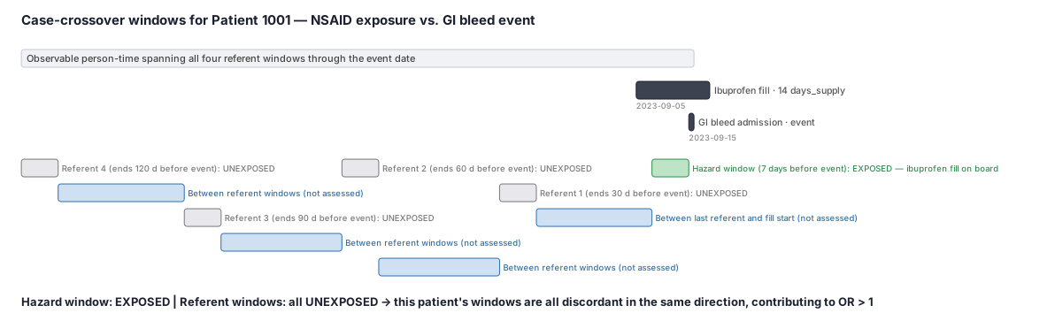
Steps
Result
OR = 4 / 1 = 4.0 — across these two patients the ibuprofen-exposure odds were four times higher in the hazard windows than in the matched referent windows, consistent with NSAID use triggering acute GI bleeding. (In a real study, hundreds of cases would be pooled via conditional logistic regression to get a stable estimate with a confidence interval.)
Trade-offs
Runnable example
Build case/referent person-period rows from claims and fit conditional logistic regression. Required inputs (cleaned, de-duplicated): events : one acute event per person -> person_id, event_date (datetime) rx : pharmacy fills -> person_id, fill_date (datetime), days_supply (int) # exposure of interest only enroll :...
import numpy as np
import pandas as pd
import statsmodels.api as sm

HAZARD_DAYS = 7          # length of each window
REFERENT_LAGS = [30, 60, 90, 120]  # days before event_date at which each referent window ENDS
GRACE = 3                # days_supply grace to bridge late refills

def _covered(days_set: set, win_end, win_len=HAZARD_DAYS) -> int:
    """1 if any exposed day falls inside the window [win_end - win_len + 1, win_end]."""
    win = {win_end - pd.Timedelta(days=d) for d in range(win_len)}
    return int(bool(days_set & win))

def build_case_crossover(events: pd.DataFrame, rx: pd.DataFrame,
                         enroll: pd.DataFrame) -> pd.DataFrame:
    # Earliest day any window can reach back to; used for the enrollment-observability check.
    earliest_lag = max(REFERENT_LAGS) + HAZARD_DAYS
    ev = events.merge(enroll, on="person_id")
    ev["covers"] = ((ev["enroll_start"] <= ev["event_date"] - pd.Timedelta(days=earliest_lag)) &
                    (ev["enroll_end"]   >= ev["event_date"]) &
                    (~ev["ma_only"]))                 # every window must be FFS-observable
    ok = ev.loc[ev["covers"], "person_id"].unique()
    ev = events[events["person_id"].isin(ok)].copy()

    # Per person, the set of calendar days covered by the exposure of interest.
    rx = rx[rx["person_id"].isin(ok)].copy()
    rx["start"] = rx["fill_date"]
    rx["end"]   = rx["fill_date"] + pd.to_timedelta(rx["days_supply"] + GRACE, unit="D")
    exposed_days = {}
    for pid, g in rx.groupby("person_id"):
        days = set()
        for _, r in g.iterrows():
            days |= {r["start"] + pd.Timedelta(days=d)
                     for d in range((r["end"] - r["start"]).days)}
        exposed_days[pid] = days

    rows = []
    for _, r in ev.iterrows():
        pid, e = r["person_id"], r["event_date"]
        days = exposed_days.get(pid, set())
        # Case window: the HAZARD_DAYS immediately before (and including) the event date.
        rows.append({"person_id": pid, "is_case_window": 1,
                     "exposed": _covered(days, e)})
        # Referent windows: each ends `lag` days before the event date (unidirectional).
        for lag in REFERENT_LAGS:
            rows.append({"person_id": pid, "is_case_window": 0,
                         "exposed": _covered(days, e - pd.Timedelta(days=lag))})
    return pd.DataFrame(rows)

def fit_case_crossover(df: pd.DataFrame):
    # Conditional logistic = stratified-by-person logit of the case-window indicator on exposure.
    model = sm.ConditionalLogit(endog=df["is_case_window"],
                                exog=df[["exposed"]],
                                groups=df["person_id"])
    res = model.fit(disp=False)
    or_ = np.exp(res.params["exposed"])
    ci = np.exp(res.conf_int().loc["exposed"])
    return res, or_, (ci[0], ci[1])
Build case/referent rows and fit conditional logistic regression with survival::clogit (the standard tool). Inputs mirror the Python version: events : person_id, event_date (Date) rx : person_id, fill_date (Date), days_supply (integer) # exposure of interest only enroll : person_id, enroll_start, enroll_end, ma_only...
library(data.table)
library(survival)

HAZARD_DAYS  <- 7L
REFERENT_LAGS <- c(30L, 60L, 90L, 120L)  # days before event_date at which each referent window ENDS
GRACE        <- 3L

build_case_crossover <- function(events, rx, enroll) {
  setDT(events); setDT(rx); setDT(enroll)
  earliest_lag <- max(REFERENT_LAGS) + HAZARD_DAYS

  # Keep only people FFS-observable across every window (no MA-only person-time).
  ev <- merge(events, enroll, by = "person_id")
  ok <- ev[enroll_start <= event_date - earliest_lag &
           enroll_end   >= event_date & !ma_only, unique(person_id)]
  ev <- events[person_id %in% ok]
  rx <- rx[person_id %in% ok]

  # Per-person set of exposed calendar days from [fill_date, fill_date + days_supply + grace).
  exposed_days <- rx[, .(day = unlist(Map(function(s, n) s + seq_len(n) - 1L,
                                          fill_date, days_supply + GRACE))),
                     by = person_id]

  covered <- function(pid, win_end) {
    win <- win_end - (0:(HAZARD_DAYS - 1L))
    as.integer(nrow(exposed_days[person_id == pid & day %in% win]) > 0L)
  }

  out <- rbindlist(lapply(seq_len(nrow(ev)), function(i) {
    pid <- ev$person_id[i]; e <- ev$event_date[i]
    case <- data.table(person_id = pid, is_case_window = 1L, exposed = covered(pid, e))
    refs <- rbindlist(lapply(REFERENT_LAGS, function(lag)
      data.table(person_id = pid, is_case_window = 0L, exposed = covered(pid, e - lag))))
    rbind(case, refs)
  }))
  out[]
}

fit_case_crossover <- function(df) {
  # Conditional logistic regression stratified on person; exp(coef) is the OR.
  clogit(is_case_window ~ exposed + strata(person_id), data = df)
}
Build case/referent person-period rows and fit conditional logistic regression with PROC LOGISTIC + STRATA (the true conditional likelihood for matched sets). Required inputs (post data-management): work.events : person_id, event_date work.rx : person_id, fill_date, days_supply /* exposure of interest only */...
%let hazard = 7;     /* window length (days)                          */
%let grace  = 3;     /* days_supply grace                             */

/* Keep only people FFS-observable back through the earliest referent window (no MA-only person-time). */
proc sql;
  create table eligible as
  select e.person_id, e.event_date
  from work.events e
  where exists (
    select 1 from work.enroll n
    where n.person_id = e.person_id and n.ma_only = 0
      and n.enroll_start <= e.event_date - (120 + &hazard)
      and n.enroll_end   >= e.event_date );
quit;

/* Per-person exposed calendar days from [fill_date, fill_date + days_supply + grace). */
data exposed_days;
  set work.rx;
  do offset = 0 to (days_supply + &grace - 1);
    exp_day = fill_date + offset;
    output;
  end;
  keep person_id exp_day;
run;
proc sort data=exposed_days nodupkey; by person_id exp_day; run;

/* One case window + four referent windows per person; exposed=1 if any exposed day falls in the window. */
data windows;
  set eligible;
  array lags[5] _temporary_ (0 30 60 90 120);   /* 0 = case window; others = referent end-lags */
  do k = 1 to 5;
    is_case_window = (k = 1);
    win_end = event_date - lags[k];
    output;
  end;
  keep person_id event_date is_case_window win_end;
run;

proc sql;
  create table cc as
  select w.person_id, w.is_case_window,
         (case when exists (
             select 1 from exposed_days d
             where d.person_id = w.person_id
               and d.exp_day between w.win_end - (&hazard - 1) and w.win_end )
            then 1 else 0 end) as exposed
  from windows w;
quit;

/* Conditional logistic regression: matched set = person_id. */
proc logistic data=cc;
  strata person_id;
  model is_case_window(event='1') = exposed;
  /* exp(estimate) for EXPOSED = transient-effect odds ratio; add /sensitivity windows in reruns. */
run;
Citations
- [1]Maclure M. The case-crossover design: a method for studying transient effects on the risk of acute events. American Journal of Epidemiology. 1991;133(2):144-153.
- [2]Maclure M, Mittleman MA. Should we use a case-crossover design? Annual Review of Public Health. 2000;21:193-221.
- [3]Mittleman MA, Maclure M, Robins JM. Control sampling strategies for case-crossover studies: an assessment of relative efficiency. American Journal of Epidemiology. 1995;142(1):91-98.