Nested Case-Control Design

In plain language

A nested case-control study starts with a group of patients who are all followed over time (a cohort), and instead of studying everyone in full detail, it zooms in only on patients who develop the outcome of interest (the cases) plus a small handful of carefully chosen comparison patients. For each case, comparison patients — called controls — are drawn from the people in the cohort who were still being followed and had not yet had the outcome at the exact moment the case was diagnosed (called the risk set). This approach gives researchers roughly the same answer as studying the whole cohort, but at a fraction of the cost — because expensive measurements like lab tests, chart reviews, or genetic assays only need to be done for the cases and their matched controls, not for everyone.

The nested case-control (NCC) design is a sampling strategy inside a fully enumerated cohort, not a stand-alone case-control study. The cohort and its person-time are defined first (entry, exit, outcome). Then, instead of measuring an expensive exposure or confounder on everyone, the analyst ascertains it only on all cases plus a small number of controls sampled from the set of cohort members still at risk at the moment each case fails (the risk set). Because controls are drawn from the same source population and the same calendar/age/follow-up structure that generated the cases, the design preserves the cohort's internal validity while collapsing the measurement burden to roughly (number of cases) x (1 + controls per case). It is the design of choice when the outcome is rare and the exposure assay is costly: stored-biospecimen biomarkers, genotyping, manual chart abstraction, NLP over clinical notes, or expert outcome adjudication.

Core conceptual distinction

The estimand and its validity hinge entirely on how controls are sampled in time, and this is the axis reviewers test. (1) Incidence-density (risk-set) sampling selects controls from those alive, enrolled, and event-free at the case's event time; matching on time means the conditional-logistic odds ratio estimates the hazard (rate) ratio of the underlying Cox model directly, with no rare-disease assumption required (Goldstein & Langholz; Lubin & Gail). Under density sampling a sampled control may later become a case and may even serve as a control for an earlier case — this is correct, not double-counting, and analyses that purge such subjects reintroduce bias. (2) Cumulative (exclusive) sampling draws controls only from those who never become cases over follow-up; the resulting odds ratio estimates the cumulative-incidence (risk) odds ratio and approximates the risk ratio only under the rare-disease assumption. Modern pharmacoepidemiology defaults to density sampling. Separately, any matching factor (age, sex, calendar time, cohort-entry date, follow-up time) is controlled by design but consumed: its main effect cannot be estimated from the matched data, and matching on a mediator or collider is the classic NCC trap.

Pros, cons, and trade-offs

- vs full-cohort Cox proportional hazards (the key comparison): NCC's only advantage is measurement cost. With expensive exposure ascertainment (biobank assays, chart review, genotyping), NCC delivers ~90% of full-cohort efficiency at 4-5 controls per case (Goldstein & Langholz) for a small fraction of the assay budget. When exposure is already cheap and universal — i.e., ordinary claims/EHR where the drug, diagnosis, and covariates sit in the data for everyone — NCC throws away information and full-cohort Cox dominates on efficiency. Choosing NCC for cheap-exposure claims data is a common and indefensible mistake. - vs case-cohort design: Both subsample a cohort, but the case-cohort comparator is a single random subcohort fixed at baseline, reusable across multiple outcomes and supporting absolute-risk estimation with weighting. NCC re-samples controls per-outcome at each event time, is more efficient for a single time-matched analysis, but the control set is outcome-specific and not naturally reusable. Prefer case-cohort for multi-outcome biobank studies; prefer NCC for one time-to-event outcome with strong time confounding (Wacholder). - vs ordinary (population) case-control: NCC fixes the source-population and selection problems of population case-control because controls are provably from the cohort that generated the cases; there is no separate, possibly incomparable, control series. - vs self-controlled designs (SCCS, case-crossover): Those eliminate all time-fixed confounding by within-person comparison but require transient, reversible exposures and recurrent or acute outcomes. NCC handles chronic exposures and between-person confounders via matching and adjustment, at the cost of residual unmeasured between-person confounding.

When to use

A rare time-to-event outcome in a defined cohort where the exposure or a key confounder is expensive to measure and you want the cohort rate ratio without assaying everyone; studies needing tight control of strong time-related confounders (age, calendar period, duration of follow-up) via matching; adjudicated-outcome or biomarker studies layered onto registries or linked claims-EHR. Use incidence-density sampling matched on the time axis and analyze with conditional logistic regression (or equivalently a Cox model on the sampled risk sets).

When NOT to use - and when it is actively misleading or dangerous

- Cheap, complete exposure in claims/EHR. If the exposure and confounders are already captured for the whole cohort, NCC is strictly less efficient than full-cohort Cox and offers no benefit; using it discards data and inflates variance. - Cumulative sampling reported as a rate ratio. Estimating the OR from exclusive (non-case) controls and presenting it as a hazard/rate ratio without the rare-disease assumption is a quantitative error; if the outcome is common the bias is large. - Time-varying exposure mis-anchored. For each matched set, exposure must be evaluated as of the index (case event) time for cases AND controls. Carrying a control's exposure forward to the case's event date, or evaluating a control's exposure at its own (later) censoring date, is a frequent macro bug that biases the rate ratio. - Over-matching. Matching on a factor on the causal pathway (a mediator) or on a collider attenuates or distorts the true effect; the matched main effect is then uninterpretable. - Differential outcome surveillance by exposure. Because the outcome defines the case set, exposure-dependent surveillance (more testing in treated patients) is amplified, not diluted, by the design.

Data-source operational depth

- Claims (FFS): Build the cohort and person-time first (continuous enrollment, washout, index/time-zero). For each case, sample controls at risk at the case's event date matched on age, sex, calendar quarter, and cohort-entry date; ascertain the expensive item (e.g., adjudicated outcome via chart pull, or a covariate requiring linkage) only on the sampled set. Lag exposure to respect induction/latency. Failure modes: Medicare Advantage person-time lacks fee-for-service claims, so MA enrollees are invisible to the risk set and sampling probabilities are distorted — restrict the risk set to FFS-observable person-time (Parts A/B/D). Stockpiling and 90-day mail-order distort `days_supply`-based exposure windows. - EHR: Risk-set membership requires the patient to be "active" (an encounter window) at the case's event time; visit-driven capture means a patient who leaves the system is not truly at risk and should not be sampled — define an observability window, not mere presence in the database. Notes/labs are the very assets NCC makes affordable to abstract. - Registry: Excellent for adjudicated outcomes and disease severity but typically incomplete for exposure; NCC is ideal when the registry case set is fixed and exposure must be pulled from linked claims or stored specimens for cases + sampled controls only. - Linked claims-EHR-vital records: The ideal substrate — EHR severity, claims completeness, reliable mortality for the competing-risk of death. Competing risks bite hardest in elderly cohorts: a potential control who died before the case's event time is no longer at risk and is ineligible for that risk set; if mortality differs by exposure, naive control sampling biases the rate ratio, so the death index must drive risk-set eligibility.

Worked claims example

Question: rate of hospitalized acute kidney injury (AKI) among new users of a nephrotoxic oral agent in 100% Medicare FFS. (1) Cohort: adults >=66 with 365 days continuous A/B/D enrollment and no prior AKI; `index_date` = first qualifying `fill_date`; follow person-time from index to first AKI (`dx` in a validated inpatient algorithm), disenrollment, death, or data end. (2) Cases: each first AKI hospitalization; its admission date is the event time. (3) Risk-set (density) sampling: for each case, randomly draw 4 controls from cohort members who at that exact event date are still enrolled, event-free, and alive, matched on age (+/-2y), sex, and calendar quarter of cohort entry. A control sampled here may itself develop AKI later and appear as a case — keep it. (4) Exposure: cumulative `days_supply` of the agent as of the matched index time, lagged 30 days for induction; ascertained identically for the case and its 4 controls as of that index time (never the control's own later date). (5) Covariate (the "expensive" item justifying NCC): baseline serum creatinine / eGFR pulled from linked lab data only for the ~5x(#cases) sampled subjects. (6) Analysis: conditional logistic regression stratified on matched set, exposure as the primary term plus eGFR and key comorbidities; the conditional OR is read as the AKI rate ratio. (7) Sensitivity: vary controls-per-case (1, 4, 10), the induction lag (0, 30, 60 days), and a negative-control outcome to probe residual confounding.

Worked example

Scenario

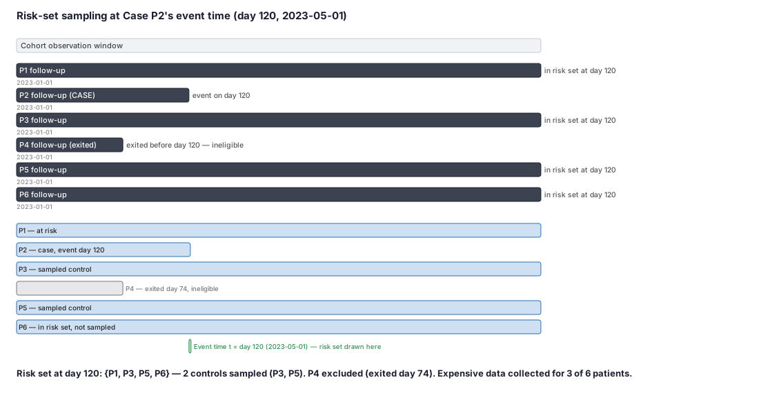
Imagine a cohort of six patients who enroll in a drug-safety study on 2023-01-01 and are followed until the end of 2023. On day 120 (2023-05-01), Patient P2 is hospitalized for the outcome we are tracking. We want to understand whether a certain exposure is linked to that hospitalization without measuring everyone's costly lab values. Using risk-set sampling, we identify which patients were still being followed and had not yet had the event on 2023-05-01, and we draw two of them as controls for P2.

Dataset

Cohort follow-up table — one row per patient, showing enrollment start, last observed date, and whether/when the outcome event occurred.

Steps

• P2 is the case: their event happens on day 120, which is 2023-05-01.

• To form the risk set on 2023-05-01, we ask: who else in the cohort was still enrolled (entry_date <= 2023-05-01), still being followed (exit_date >= 2023-05-01), and had not yet had the event? That gives us P1, P3, P5, and P6.

• P4 is excluded from the risk set because their last observed date was 2023-03-15 — they had already left the study before P2's event date.

• We randomly sample 2 controls from the eligible risk set {P1, P3, P5, P6}. Say we draw P3 and P5.

• The matched set for P2 is now: one case (P2) plus two controls (P3, P5), all anchored to the same event date of 2023-05-01.

• Expensive measurements (lab values, chart data) are collected only for P2, P3, and P5 — 3 patients instead of all 6.

• If additional cases occur later in follow-up, the same process repeats at each new event time. Note that P3 or P5 could themselves become cases later and appear in a future matched set as cases — that is correct and expected.

Result

Risk-set sampling reduces measurement to 3 of 6 cohort members (50%) for this event, and approaches 5 of 6 savings (roughly 80-90% cost reduction) in large studies with rare outcomes and 4-5 controls per case — without meaningfully sacrificing the accuracy of the rate estimate.

Timeline Spec

Title

Risk-set sampling at Case P2's event time (day 120, 2023-05-01)

Window

Start

2023-01-01

End

2023-12-31

Label

Cohort observation window

Events

• Label

  P1 follow-up

  Start

  2023-01-01

  Length Days

  365

  Quantity

  in risk set at day 120

• Label

  P2 follow-up (CASE)

  Start

  2023-01-01

  Length Days

  120

  Quantity

  event on day 120

• Label

  P3 follow-up

  Start

  2023-01-01

  Length Days

  365

  Quantity

  in risk set at day 120

• Label

  P4 follow-up (exited)

  Start

  2023-01-01

  Length Days

  74

  Quantity

  exited before day 120 — ineligible

• Label

  P5 follow-up

  Start

  2023-01-01

  Length Days

  365

  Quantity

  in risk set at day 120

• Label

  P6 follow-up

  Start

  2023-01-01

  Length Days

  365

  Quantity

  in risk set at day 120

Spans

• Kind

  followup

  Start

  2023-01-01

  End

  2023-12-31

  Label

  P1 — at risk

• Kind

  followup

  Start

  2023-01-01

  End

  2023-05-01

  Label

  P2 — case, event day 120

• Kind

  followup

  Start

  2023-01-01

  End

  2023-12-31

  Label

  P3 — sampled control

• Kind

  unexposed

  Start

  2023-01-01

  End

  2023-03-15

  Label

  P4 — exited day 74, ineligible

• Kind

  followup

  Start

  2023-01-01

  End

  2023-12-31

  Label

  P5 — sampled control

• Kind

  followup

  Start

  2023-01-01

  End

  2023-12-31

  Label

  P6 — in risk set, not sampled

• Kind

  exposed

  Start

  2023-05-01

  End

  2023-05-01

  Label

  Event time t = day 120 (2023-05-01) — risk set drawn here

Markers

• Date

  2023-05-01

  Label

  Case P2 event — risk set sampled at this moment

Result

Label

Risk set at day 120: {P1, P3, P5, P6} — 2 controls sampled (P3, P5). P4 excluded (exited day 74). Expensive data collected for 3 of 6 patients.

Value

0.5

Caption

Each horizontal bar shows one patient's follow-up period. The vertical line at day 120 (2023-05-01) marks when P2 had the event. Controls are drawn only from patients whose bars cross that line and who have not yet had the event — the risk set. P4's bar ends before day 120, so they are ineligible.

Alt Text

Six horizontal patient follow-up bars on a 2023 timeline. A vertical marker at day 120 (May 1) shows the case event time for P2. Bars for P1, P3, P5, and P6 extend past that line, forming the risk set. P4's bar ends at day 74, before the marker, making them ineligible. P3 and P5 are highlighted as the sampled controls.

Runnable example

import numpy as np
import pandas as pd
from statsmodels.discrete.conditional_models import ConditionalLogit

N_CONTROLS = 4
rng = np.random.default_rng(20240101)

def sample_risk_sets(cohort: pd.DataFrame, match_cols=("sex", "age_band")) -> pd.DataFrame:
    cases = cohort[cohort["event"] == 1]
    rows = []
    for _, case in cases.iterrows():
        t = case["event_date"]
        # At-risk at t: entered on/before t, still under observation at t (alive, enrolled, event-free at t).
        at_risk = cohort[(cohort["entry_date"] <= t) & (cohort["exit_date"] >= t) &
                         (cohort["person_id"] != case["person_id"])]
        for c in match_cols:                      # exact matching on time-stable factors
            at_risk = at_risk[at_risk[c] == case[c]]
        k = min(N_CONTROLS, len(at_risk))
        ctrl = at_risk.sample(k, random_state=int(rng.integers(1e9))) if k else at_risk
        rows.append({"set_id": case["person_id"], "person_id": case["person_id"],
                     "index_time": t, "is_case": 1})
        for pid in ctrl["person_id"]:
            rows.append({"set_id": case["person_id"], "person_id": pid,
                         "index_time": t, "is_case": 0})
    return pd.DataFrame(rows)

sets = sample_risk_sets(cohort)
# Attach exposure measured AS OF index_time for every member (case and controls alike), then model.
sets = sets.merge(expo, on="person_id", how="left")   # expo computed at each row's index_time upstream
m = ConditionalLogit(sets["is_case"], sets[["cum_days_supply"]], groups=sets["set_id"]).fit()
print(m.summary())   # exp(coef) is the rate (hazard) ratio under density sampling

library(data.table)
library(survival)
N_CONTROLS <- 4L
set.seed(20240101)

sample_risk_sets <- function(cohort) {
  setDT(cohort)
  cases <- cohort[event == 1L]
  out <- vector("list", nrow(cases))
  for (i in seq_len(nrow(cases))) {
    ca <- cases[i]
    t  <- ca$event_date
    # At-risk at t and matched on time-stable factors; exclude the case itself.
    pool <- cohort[entry_date <= t & exit_date >= t & person_id != ca$person_id &
                   sex == ca$sex & age_band == ca$age_band]
    k <- min(N_CONTROLS, nrow(pool))
    ctrl <- if (k > 0L) pool[sample(.N, k)] else pool
    out[[i]] <- rbind(
      data.table(set_id = ca$person_id, person_id = ca$person_id, index_time = t, is_case = 1L),
      data.table(set_id = ca$person_id, person_id = ctrl$person_id, index_time = t, is_case = 0L)
    )
  }
  rbindlist(out)
}

sets <- sample_risk_sets(cohort)
sets <- merge(sets, expo, by = "person_id")          # cum_days_supply as of index_time
fit <- clogit(is_case ~ cum_days_supply + strata(set_id), data = sets)
summary(fit)   # exp(coef) = rate ratio