Competing Risks (Cause-Specific Hazard, Cumulative Incidence, and Fine-Gray)

In plain language

Competing-risks analysis asks: what is the true probability that a patient experiences a specific bad outcome — like a severe infection — before something else (such as death) gets in the way first? Standard survival curves pretend that patients who die can still go on to have the infection later, which inflates the estimated risk. Competing-risks methods keep track of two types of outcomes at once and report the honest probability that the infection actually occurs. Two regression tools help: one focuses on the rate of the infection among patients who are still alive and infection-free (cause-specific hazard), and one ties its estimate directly to that honest probability curve (Fine-Gray model).

A competing risk is an event whose occurrence precludes the event of interest (EOI) from ever happening, or fundamentally changes its probability and interpretation: death before a hospitalization, next-line therapy before documented progression, transplant before dialysis-related death, prosthesis revision before a readmission. The defining feature is that, once the competing event occurs, the patient is no longer at risk for the EOI in any meaningful sense — a dead patient cannot be hospitalized. The single most consequential and most common error in real-world time-to-event analysis is treating a competing event as if it were ordinary independent (administrative) censoring, which is what every default `survfit`/Kaplan-Meier/Cox call does unless you intervene.

Core estimand distinction — three quantities, three questions

- Cause-specific hazard. Among patients still free of both the EOI and any competing event, the instantaneous rate at which the EOI occurs. It answers an etiologic/mechanistic question ("does the drug change the biology of progression among those still able to progress?"). Competing events are treated as censoring in the partial likelihood. A standard Cox model with the competing event coded as censored estimates the cause-specific hazard ratio. - Cumulative incidence function (CIF), a.k.a. subdistribution function. The actual probability that a patient experiences the EOI before any competing event by time t. This is the decision-relevant, patient- and payer-facing number — the quantity that belongs in a label, an HTA dossier, or a risk calculator. It is estimated non-parametrically by the Aalen-Johansen estimator. Crucially, CIF_EOI(t) + CIF_competing(t) + S(t) = 1, so the EOI incidence is bounded by the room the competing event leaves it. The complement of Kaplan-Meier (1 − KM) over-states this probability because it implicitly assumes patients removed by the competing event could still go on to have the EOI. - Fine-Gray subdistribution hazard. A proportional-hazards regression whose coefficient maps monotonically onto the CIF: a subdistribution HR > 1 means a higher cumulative incidence. It achieves this by keeping subjects who experience the competing event in an "extended" risk set (with decreasing weight over time) rather than removing them. The price is interpretive: the subdistribution HR is not a biological rate and must never be described as "the hazard among those still able to have the event."

The trap that makes all three necessary

The cause-specific HR and the subdistribution HR can point in opposite directions for the same exposure. A drug that strongly reduces non-cancer mortality leaves more patients alive and at risk to progress; its cause-specific HR for progression may be ~1, while its subdistribution HR for progression is > 1 (more progression events accrue simply because fewer people die first). Neither is "wrong" — they answer different questions. This is why best practice (Austin & Fine 2017; Latouche et al.) is to pre-specify the primary estimand in the protocol/SAP and to report the CIF curves plus both regression models so reviewers can see the mechanism.

Pros, cons, and trade-offs

- vs. 1 − Kaplan-Meier / Cox with competing events censored (the naive default). The competing-risks approach yields honest absolute risk: it never lets the EOI incidence exceed the room left by competing mortality, so it avoids overstating benefit (e.g., "stroke prevention" in a frail population that mostly dies of other causes) or harm. Cost: more complex to code and to explain, and the numbers are typically lower than the 1−KM curves clinicians expect, which generates pushback. Prefer competing-risks whenever a competing event is common (rule of thumb: cumulative competing incidence > ~10%) or differs across exposure arms. A plain Cox cause-specific analysis is defensible only when the competing event is rare and balanced and the question is genuinely about the conditional rate. - Cause-specific Cox vs. Fine-Gray. Cause-specific is the right tool for etiology and is unbiased for the rate among those at risk; it is trivial to fit (any Cox engine) and its covariate effects on multiple causes combine coherently. Fine-Gray is the right tool when the deliverable is the probability you will plot and quote, because its coefficient is tied to that curve. The trade-off: Fine-Gray HRs lose mechanistic meaning and can be unstable when the competing event dominates; cause-specific HRs require a separate standardization/Aalen-Johansen step to recover absolute risk. Modern guidance: report cause-specific HRs for each cause and the CIF; add Fine-Gray when a single covariate-adjusted statement about the EOI probability is the headline. - vs. RMST / restricted mean time lost. The CIF answers "what fraction by time t"; RMST-type summaries answer "how much event-free time" in interpretable time units and can be extended to competing risks (mean time lost to each cause). They are complements, often reported together for HTA.

When to use

Any RWE time-to-event analysis in a population with non-trivial competing mortality or terminal intercurrent events: oncology (progression/discontinuation competing with death and next-line therapy), cardiology and nephrology in the elderly (non-CV death), device/procedure studies (revision, reoperation, death), transplant, and any HTA or label-supporting estimate of absolute incidence. It is the default whenever the deliverable is a probability and death is on the table.

When NOT to use — and when censoring the competing event is actively misleading

- Do not 1 − KM a competing event. If you report a 1 − KM curve for hospitalization while ignoring that 18% of the cohort died first, the curve is an artifact of an impossible counterfactual world and will overstate incidence — the more so the higher and more differential the competing mortality. This is the single dangerous mistake the method exists to prevent. - Do not interpret a subdistribution HR as a rate. Reporting "the Fine-Gray HR shows the drug halves the hazard of progression" is wrong; it concerns the cumulative incidence, not a hazard among the at-risk. - Do not Fine-Gray when the competing event itself is the scientific target of a mechanistic claim — use cause-specific models for each cause and let the CIFs carry the absolute story. - Do not conflate informative administrative censoring with competing risks. Disenrollment that depends on prognosis is dependent censoring, handled by IPCW, not by recoding it as a competing event; mixing the two double-counts the correction.

Data-source operational depth

- Claims (FFS vs. Medicare Advantage). Build mutually exclusive first-event dates for the EOI and each competing event on the same observable follow-up window, then code one event type per person from `min(eoi_date, competing_date, censor_date)`. Death is the dominant competing risk in elderly/oncology RWE and is the hardest to get right: discharge status (`disch_status`) captures only in-hospital death and undercounts out-of-hospital death — link to a mortality file (Medicare enrollment/EDB date of death, SSDMF where still available, or state vital records). Medicare Advantage person-time lacks adjudicated FFS claims, so both EOI events and deaths are differentially missing for MA enrollees; either restrict to FFS A/B (plus D for exposure) or use an MA-aware death source, because differential ascertainment of the competing event by arm is exactly what flips the cause-specific vs. subdistribution contrast. Disenrollment is administrative censoring, handled separately (IPCW if informative), never recoded as a competing event. - EHR. Progression/recurrence dates frequently live in notes or tumor-registry linkage, not structured fields; death is badly undercaptured because patients who die out-of-system simply stop appearing (loss to follow-up masquerading as event-free survival). Visit-driven capture adds interval censoring on top of the competing-risk structure. Link to claims and a death index before trusting any CIF. - Registry. Usually the best source for adjudicated cause-specific death, recurrence, and progression; still link to claims for complete pharmacy exposure timing and out-of-system HCRU that competes. - Linked claims–EHR–vital records. The ideal substrate (severity + completeness + reliable mortality) but linkage selection and order/fill/service date discrepancies must be reconciled before first-event coding, or the "first event" can be assigned to the wrong cause.

Worked claims example

Question: 12- and 24-month cumulative incidence of a first inpatient febrile-neutropenia (FN) admission after initiating a new line of cytotoxic chemotherapy, comparing regimen A vs. regimen B, in a Medicare FFS oncology cohort. (1) Eligibility: age ≥66, a qualifying cancer diagnosis, and 365 days of continuous Part A/B enrollment before the index regimen (washout that also makes both arms incident users of that line). (2) Index/time zero: date of the first administration claim (J-code) for regimen A or B; assign the arm from that claim. (3) Event of interest: first inpatient admission with an FN diagnosis (`dx` in the validated FN code set) on a facility claim, `event_type = 1`. (4) Competing event: all-cause death from the Medicare enrollment date-of-death field — not discharge status alone, which misses out-of-hospital deaths — `event_type = 2`. (5) First-event coding: for each person, `fu_time = min(fn_date, death_date, censor_date) − index_date` and `event_type` is the cause that achieved that minimum; ties broken by a pre-specified rule. (6) Censoring (`event_type = 0`): disenrollment from FFS, transition to MA-only (FFS claims stop, so FN can no longer be observed — treat as administrative censoring, not as event-free), and end of data. (7) Estimate: arm-stratified Aalen-Johansen CIF reported at 12 and 24 months with 95% CIs; a 1 − KM curve for FN would over-state incidence because the ~15–25% who die first cannot then be hospitalized. (8) Regression: cause-specific Cox (death censored) for the etiologic effect on FN rate and a Fine-Gray model for the effect on the FN probability; if regimen A causes more early death, expect the two HRs to diverge, and the CIF curves explain why. (9) Sensitivity: vary the FN code set, the death source (enrollment field vs. claims-based), and tie-breaking, and check whether differential competing mortality across arms drives any divergence.

Interpreting the output

For febrile neutropenia (FN) in a chemotherapy trial: cause-specific HR = 0.68 (arm A vs B) and Fine-Gray subdistribution HR = 0.79 for the same endpoint in the same dataset.

Formal interpretation. The cause-specific HR (0.68) removes patients who die before FN from the risk set at each event time and estimates how quickly FN accrues among survivors; it answers the etiologic question of whether arm A genuinely reduces the biological rate of FN. The Fine-Gray subdistribution HR (0.79) retains all patients — including those who died — in a subdistribution risk set and directly models the cumulative incidence function; it answers the predictive question of how much lower the absolute probability of ever experiencing FN is on arm A. The two quantities diverge whenever competing mortality differs between arms. Neither is wrong; they answer different scientific questions.

Practical interpretation. If arm A also causes more early death, dead patients cannot develop FN, compressing the FN cumulative incidence even if the underlying biology is unchanged. Report the Aalen-Johansen CIF alongside both HRs. For clinical decision-making about infection risk, use the Fine-Gray model and CIF; for mechanistic understanding of whether the drug suppresses neutropenia biology, use the cause-specific HR.

Worked example

Scenario

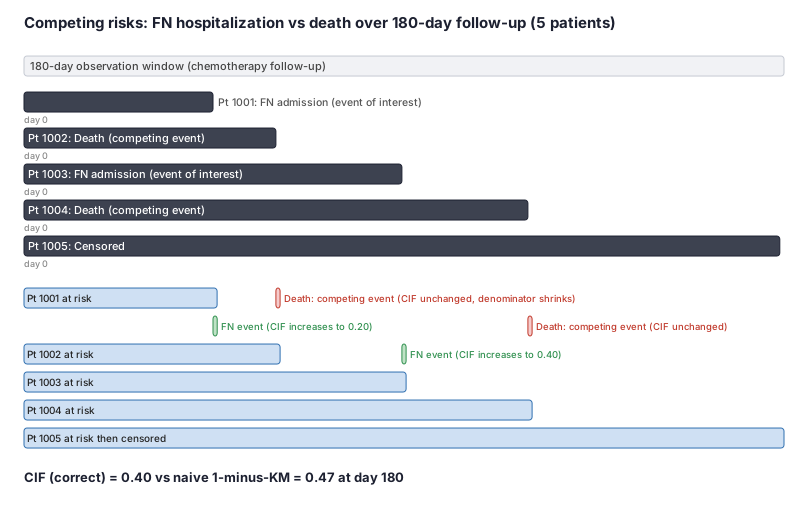
Five Medicare patients start a new chemotherapy regimen on Day 0. We want to know the 6-month (180-day) probability of a first febrile-neutropenia (FN) hospitalization. Some patients have the FN admission (event of interest); others die before any FN occurs (competing event); one is still event-free at day 180 (censored). We compare the naive Kaplan-Meier estimate — which wrongly treats death as ordinary censoring — with the correct cumulative incidence function that accounts for competing mortality.

Dataset

One-row-per-patient analytic table: follow-up time and outcome type for five Medicare FFS patients.

Steps

• Order all five patients by their follow-up time: 45, 60, 90, 120, 180 days.

• At each event time, note how many patients are still in the risk set (have not yet had any event or been censored).

• Naive Kaplan-Meier ignores the event type and treats both FN and death as 'events' for a combined curve, or — the common error — treats death as censoring when estimating FN risk.

• If death is censored naively: at day 45 (patient 1001, FN), risk set = 5, KM drops by 1/5 = 0.20; at day 90 (patient 1003, FN), risk set appears to be 3 (patients 1002 and 1004 were wrongly 'censored'), KM drops by 1/3 = 0.33.

• Naive 1-minus-KM probability of FN by day 180 = 1 - (4/5)(2/3) = 1 - 0.533 = 0.467, or about 47%.

• The correct cumulative incidence function (CIF) uses the Aalen-Johansen estimator, which keeps competing deaths in the denominator of the risk set but does NOT let them count as FN events.

• At day 45 (FN): risk set = 5, CIF increases by (1/5) x current overall survival = 0.20 x 1.0 = 0.200.

• At day 60 (death): risk set = 4, no change to the FN CIF; overall survival drops to 3/4 x 0.80 = 0.600.

• At day 90 (FN): risk set = 3, CIF increases by (1/3) x 0.600 = 0.200; cumulative FN CIF = 0.200 + 0.200 = 0.400.

• At day 120 (death): no change to FN CIF; overall survival drops further. Patient 1005 censored at day 180.

Result

Correct cumulative incidence of FN by day 180 = 0.40 (40%). Naive 1-minus-KM = 0.47 (47%). The naive approach overstates FN risk by 7 percentage points because it pretends the two patients who died could still go on to have an FN admission — but dead patients cannot be hospitalized.

Timeline Spec

Title

Competing risks: FN hospitalization vs death over 180-day follow-up (5 patients)

Window

End Day

180

Label

180-day observation window (chemotherapy follow-up)

Events

• Label

  Pt 1001: FN admission (event of interest)

  End Day

  45

  Marker

  FN hospitalization at day 45

• Label

  Pt 1002: Death (competing event)

  End Day

  60

  Marker

  Death at day 60

• Label

  Pt 1003: FN admission (event of interest)

  End Day

  90

  Marker

  FN hospitalization at day 90

• Label

  Pt 1004: Death (competing event)

  End Day

  120

  Marker

  Death at day 120

• Label

  Pt 1005: Censored

  End Day

  180

  Marker

  Censored at day 180 (end of window)

Spans

• Kind

  followup

  End Day

  45

  Label

  Pt 1001 at risk

• Kind

  covered

  Start Day

  45

  End Day

  45

  Label

  FN event (CIF increases to 0.20)

• Kind

  followup

  End Day

  60

  Label

  Pt 1002 at risk

• Kind

  gap

  Start Day

  60

  End Day

  60

  Label

  Death: competing event (CIF unchanged, denominator shrinks)

• Kind

  followup

  End Day

  90

  Label

  Pt 1003 at risk

• Kind

  covered

  Start Day

  90

  End Day

  90

  Label

  FN event (CIF increases to 0.40)

• Kind

  followup

  End Day

  120

  Label

  Pt 1004 at risk

• Kind

  gap

  Start Day

  120

  End Day

  120

  Label

  Death: competing event (CIF unchanged)

• Kind

  followup

  End Day

  180

  Label

  Pt 1005 at risk then censored

Result

Label

CIF (correct) = 0.40 vs naive 1-minus-KM = 0.47 at day 180

Cif Value

0.4

Naive Km Value

0.47

Overstatement

0.07

Caption

Each horizontal bar shows one patient's follow-up from Day 0 to their first event or censoring. Orange markers indicate febrile-neutropenia admissions (event of interest); red markers indicate deaths (competing events). The correct cumulative incidence function (CIF = 0.40) is lower than the naive Kaplan-Meier estimate (0.47) because deaths are kept in the denominator of the risk set without inflating the FN numerator.

Alt Text

Five horizontal patient timelines from Day 0 to Day 180. Patients 1001 and 1003 end with orange FN-event markers at days 45 and 90. Patients 1002 and 1004 end with red death markers at days 60 and 120. Patient 1005 reaches day 180 with a censoring mark. Below the timelines, a stepped CIF curve rises to 0.40 while a dashed naive KM curve rises higher to 0.47, illustrating the overstatement when deaths are incorrectly treated as censored.

Runnable example

import pandas as pd
from lifelines import AalenJohansenFitter, CoxPHFitter

EOI = 1            # event of interest
HORIZONS = [365, 730]   # 12 and 24 months, in days

def cif_by_arm(cohort: pd.DataFrame, horizons=HORIZONS) -> pd.DataFrame:
    """Aalen-Johansen CIF of the event of interest, per arm, at fixed horizons.

    The CIF (not 1 - KM) is the honest absolute probability: competing events
    are kept out of the EOI numerator AND keep their place in the denominator,
    so EOI incidence can never exceed the room competing mortality leaves it.
    """
    rows = []
    for arm, g in cohort.groupby("arm"):
        ajf = AalenJohansenFitter(calculate_variance=True)
        # event_of_interest=1 tells lifelines which code is the EOI; all other
        # non-zero codes are handled as competing (not as censoring).
        ajf.fit(g["fu_time"], g["event_type"], event_of_interest=EOI)
        cif = ajf.cumulative_density_
        ci = ajf.confidence_interval_
        for h in horizons:
            # step function: value at the last observed time <= horizon
            at = cif.loc[cif.index <= h]
            lo = ci.loc[ci.index <= h]
            rows.append({
                "arm": arm, "horizon_days": h,
                "cif_eoi": float(at.iloc[-1, 0]) if len(at) else 0.0,
                "cif_lower": float(lo.iloc[-1, 0]) if len(lo) else 0.0,
                "cif_upper": float(lo.iloc[-1, 1]) if len(lo) else 0.0,
            })
    return pd.DataFrame(rows)

def cause_specific_cox(cohort: pd.DataFrame, covariates: list[str]) -> CoxPHFitter:
    """Cause-specific HR for the EOI: code competing events as censored (0),
    EOI as the event (1). This is the etiologic rate among those still at risk,
    NOT the probability scale -- pair it with cif_by_arm()."""
    d = cohort.copy()
    d["event"] = (d["event_type"] == EOI).astype(int)  # competing -> 0 (censored)
    cph = CoxPHFitter()
    cph.fit(d[["fu_time", "event"] + covariates], duration_col="fu_time", event_col="event")
    return cph

library(survival)
library(cmprsk)

# event_type must be a factor with the censoring level first for finegray():
d$event_f <- factor(d$event_type, levels = c(0, 1, 2),
                    labels = c("censor", "eoi", "competing"))

## 1. Non-parametric CIF by arm (Aalen-Johansen). multi-state survfit handles competing risks.
aj <- survfit(Surv(fu_time, event_f) ~ arm, data = d)
print(summary(aj, times = c(365, 730)))   # 12- and 24-month CIF, with CIs

## 2. Cause-specific Cox for the EOI: competing events are censored (status == "eoi" only).
cs_eoi <- coxph(Surv(fu_time, event_f == "eoi") ~ arm + age + sex, data = d)
summary(cs_eoi)        # cause-specific HR (etiologic rate among those at risk)

## 3. Fine-Gray subdistribution model via finegray() + coxph().
fg_data <- finegray(Surv(fu_time, event_f) ~ ., data = d, etype = "eoi")
fg <- coxph(Surv(fgstart, fgstop, fgstatus) ~ arm + age + sex,
            weights = fgwt, data = fg_data)
summary(fg)            # subdistribution HR -> maps to the CIF scale, NOT a rate

## 3b. Equivalent with cmprsk::crr (failcode = EOI, cencode = censoring code).
covs <- model.matrix(~ arm + age + sex, data = d)[, -1]
fg2 <- crr(ftime = d$fu_time, fstatus = d$event_type,
           cov1 = covs, failcode = 1, cencode = 0)
summary(fg2)