Cumulative Incidence and Absolute Risk Estimation

In plain language

Cumulative incidence answers one practical question: out of every 100 patients who started the study healthy, how many had the event by a specific point in time? You count who had the event, divide by the number of patients in the group at the very beginning, and express it as a proportion — for example, '3 out of 8 patients had a stroke within one year.' One important complication: if some patients can die from another cause before getting the event, those deaths cannot simply be ignored, because a patient who has already died can never have a stroke — counting them as though they might still get the event inflates the risk estimate.

Cumulative incidence (absolute risk)

is the probability that the event of interest has occurred by a fixed follow-up horizon t, given the subject was event-free at time zero. It is the quantity decision-makers actually want — "what is a patient's 1-year risk of stroke on this drug?" — and is the natural input to number-needed-to-treat, benefit-risk tables, cost-effectiveness Markov traces, and HTA absolute-effect framing. The estimator you choose is the entire methodological content of this concept, and choosing wrong silently biases the headline number.

Core estimand distinction — and the canonical trap

Three distinct quantities are routinely (and wrongly) conflated: - Cause-specific hazard — the instantaneous rate of the event among those still event-free and still at risk (competing events remove subjects from the risk set). This is the etiologic quantity: how the exposure acts on the biological process. A cause-specific Cox model answers "does the drug change the rate of the event?" - Cumulative incidence function (CIF) — the absolute probability of the event by time t, computed so that the CIFs for all event types plus the event-free probability sum to 1. This is the prognostic / decision quantity. With no competing risks it equals 1 − Kaplan-Meier (1−KM); with competing risks it is the Aalen-Johansen estimator, which correctly treats competing events as a separate exit, not as censoring. - Subdistribution hazard (Fine-Gray) — a regression that targets the CIF directly by keeping subjects who experienced a competing event in a modified ("subdistribution") risk set. Its hazard ratio describes the effect on absolute risk, which is what changes a benefit-risk conclusion.

The single error reviewers hunt for: using 1−KM for the event of interest when competing events are non-negligible. Kaplan-Meier censors the competing event (e.g., death) and assumes it is independent and "could have gone on to have the event." It therefore overestimates cumulative incidence, and the overestimation is differential whenever the competing-event rate differs by arm — exactly the situation in elderly claims populations where one drug's patients die faster. The sum of separate 1−KM curves across event types can exceed 1, which is the diagnostic tell that the estimator is incoherent. Use Aalen-Johansen (descriptive) and Fine-Gray (regression) for absolute risk; reserve cause-specific hazards for etiology. A complete competing-risks analysis usually reports both the cause-specific and subdistribution models, because they answer different questions and can point in opposite directions.

Pros, cons, and trade-offs

- 1−Kaplan-Meier vs Aalen-Johansen CIF: 1−KM is simpler, ubiquitous, and correct only when the competing-event rate is negligible. Aalen-Johansen costs nothing extra to compute and is always coherent (curves sum to ≤1). Prefer Aalen-Johansen for any absolute-risk statement when death or another terminal competing event is plausible (almost all elderly or oncology RWE). Use plain 1−KM only when the competing risk is truly rare or when the estimand is a composite that includes it. - Cause-specific Cox vs Fine-Gray subdistribution: the cause-specific HR is the cleaner etiologic effect and is what you want for mechanism; the Fine-Gray subdistribution HR maps to the absolute-risk effect and is what you want for prognosis and HTA. Cost: the subdistribution HR has a non-intuitive interpretation (it operates on a risk set that retains subjects who already had a competing event) and is sensitive to the competing-event rate, so it is not transportable across populations with different background mortality. Report both; do not pick one and call it "the" effect. - CIF/risk vs incidence rate (person-time): a rate (events per person-year) is a hazard summary, not a probability, and is not bounded by 1; it is the right currency when follow-up is short relative to risk or when you need a single summary across variable follow-up. Cumulative incidence is the right currency for fixed-horizon absolute risk and decision modeling. They are not interchangeable — see the incidence-rate concept. - CIF vs RMST: restricted mean survival time summarizes the whole curve up to a horizon as expected event-free time and sidesteps proportional-hazards assumptions; CIF gives the point-in-time probability. RMST is often the better single comparative summary when curves cross; CIF is what a clinician reads off for "risk by year 1."

When to use

Any fixed-horizon absolute-risk question in cohort RWE: 1-year risk of an adverse event, 5-year recurrence, cumulative incidence of a utilization or cost event; the descriptive backbone of comparative safety studies; the input layer for decision-analytic and HTA models that need absolute probabilities rather than hazard ratios.

When NOT to use / when this is actively misleading

- Do not use 1−KM for cause-specific cumulative incidence when a competing event is common. This is the dominant failure mode and it is systematic upward bias, worsened differentially by arm. Switch to Aalen-Johansen. - Do not interpret a Fine-Gray subdistribution HR as an etiologic effect — a drug can have no effect on the cause-specific hazard yet show a non-null subdistribution HR purely because it changes the competing (death) rate. - Do not report a single estimator when competing risks exist. A cause-specific HR near 1 with a Fine-Gray HR <1 is not a contradiction; it usually means the exposure reduces the competing event. Reporting only one hides the story. - Do not estimate cumulative incidence with informative/dependent censoring (e.g., disenrollment driven by the outcome) without addressing it — Aalen-Johansen and KM both assume censoring is non-informative within the modeled structure. - Immortal time. If time zero is set at a landmark that requires surviving to receive a treatment/procedure, the risk denominator is corrupted before any estimator runs; fix the cohort (see immortal-time-bias-handling), not the formula.

Data-source operational depth

- Claims (FFS vs Medicare Advantage): the at-risk denominator is observed person-time under continuous enrollment, and the dominant competing risk in older cohorts is death. Two distinct failure modes: (1) MA-only person-time lacks adjudicable FFS claims, so events and competing deaths are under-ascertained — restrict the risk set to enrollees with Parts A/B (and D for drug exposure) and exclude MA-only spans rather than treating them as event-free follow-up. (2) Death is incompletely captured in claims alone (disenrollment and death are confounded); link to the Medicare/SSA death master or vital records, otherwise the competing event is misclassified as censoring and the analysis silently collapses back to a 1−KM-like overestimate. Censor at disenrollment, end of data, and horizon; treat death as a competing event, not a censor. - EHR: capture is encounter-driven, so both the event and the competing death can be missed when a patient leaves the system — loss to follow-up is potentially informative and biases the CIF. Define the observation window explicitly, link to an external death index, and report follow-up completeness by arm. - Registry: strong for adjudicated events and (often) vital status, which makes the competing-risk structure trustworthy; typically weak for complete drug exposure and for out-of-registry events. Link to claims to firm up exposure and non-registry outcomes. - Linked claims–EHR–vital records: the ideal substrate — EHR severity for risk adjustment, claims completeness for person-time, and a reliable death index to model the competing risk — but linkage selects the linkable subset and introduces order/fill/service-date discrepancies that must be reconciled before time zero and the at-risk clock are set.

Worked claims example

Question: 1-year cumulative incidence of ischemic stroke among adults ≥66 initiating anticoagulant A vs anticoagulant B in Medicare fee-for-service, where death is a strong competing risk. (1) Eligibility: ≥66 years, ≥365 days continuous Parts A/B/D before the first qualifying fill, no anticoagulant fill in the 365-day washout (incident users of both arms). (2) Time zero: the first qualifying `fill_date`; assign arm from the NDC dispensed that day. (3) At-risk clock: from time zero, person-time accrues only while continuously enrolled in FFS (no MA-only spans). (4) Event ascertainment: first inpatient ischemic-stroke diagnosis in the primary position within the 365-day horizon. (5) Competing event: all-cause death from the linked death master file — coded as a competing event, not as censoring. (6) Other censoring: FFS disenrollment, end of data, horizon. (7) Estimate the CIF with Aalen-Johansen by arm; also compute the naive 1−KM and show it materially exceeds the CIF (e.g., 1−KM 6.1% vs CIF 5.2% in the arm with higher background mortality), with a larger gap in the older/sicker arm — that gap is the differential bias 1−KM would inject into the headline. (8) Fit a Fine-Gray model for the adjusted subdistribution HR on absolute stroke risk and a cause-specific Cox model for the etiologic rate, reporting both. (9) Sensitivity: vary the horizon, the grace period for as-treated exposure, and a death-only-from-claims definition to bound the impact of incomplete mortality capture.

Interpreting the output

An Aalen-Johansen cumulative incidence analysis returns: 12-month stroke incidence = 8.0% (95% CI 6.2–10.1%) in the treated group; naive 1−KM estimate = 9.3% — an overstatement of 1.3 percentage points driven by competing mortality.

Formal interpretation. The Aalen-Johansen CIF of 8.0% is the estimated probability of experiencing stroke by 12 months in the presence of competing risks. It treats competing events (primarily non-stroke death) as events — not as censoring — so patients who die cannot later have a stroke. The naive 1−KM estimate of 9.3% treats competing deaths as censored observations, implicitly assuming that censored patients remain at risk and would eventually have strokes at the same rate as survivors. Under competing risks this is impossible, and 1−KM therefore overstates absolute stroke probability. The magnitude of overstatement grows with the competing event rate and the length of follow-up.

Practical interpretation. The 1.3 percentage point difference between 1−KM (9.3%) and CIF (8.0%) is clinically meaningful at scale: applied to a population of 100,000 patients, it corresponds to 1,300 apparent strokes that do not exist. For regulatory benefit-risk submissions and payer-facing burden-of-disease reports, report the Aalen-Johansen CIF as the primary absolute risk estimate, pair it with a Fine-Gray regression for covariate-adjusted inference on absolute stroke risk, and report the cause-specific Cox model for the etiologic hazard.

Worked example

Scenario

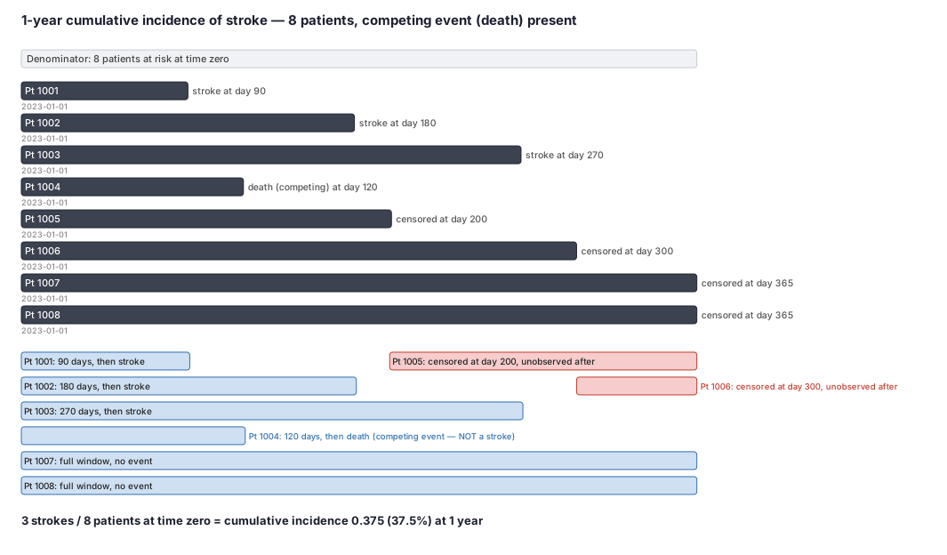
A researcher wants to know the 1-year cumulative incidence of ischemic stroke among 8 patients who started a new anticoagulant on the same day (time zero = day 0). Each patient is followed for up to 365 days. Some patients have a stroke (the event of interest), some die from another cause (a competing event — once dead, a patient cannot have a stroke), and some reach the end of follow-up without any event (censored). The question is: what fraction of the original 8 patients experienced a stroke within one year?

Dataset

One row per patient showing how long each was followed and what happened first. Status codes: 0 = censored (no event by end of follow-up), 1 = stroke (event of interest), 2 = death from another cause (competing event).

Steps

• Start with all 8 patients in the denominator — everyone who was at risk at time zero (day 0).

• Count patients who had a stroke (status = 1) by day 365: patients 1001, 1002, and 1003 — that is 3 strokes.

• Patient 1004 died from another cause at day 120 (status = 2). This is a competing event: once dead, this patient could never have had a stroke, so they are NOT counted in the stroke numerator.

• Patients 1005 and 1006 were censored before day 365 because they left the insurance plan. We know they had not had a stroke yet at that point, but we cannot observe them afterward.

• Patients 1007 and 1008 reached the end of the 365-day window with no stroke — they are also censored at day 365.

• Cumulative incidence at 365 days = strokes observed / patients at risk at time zero = 3 / 8 = 0.375, or 37.5 per 100 patients.

Result

Cumulative incidence at 1 year = 3 strokes / 8 patients at time zero = 0.375 (37.5%).

Timeline Spec

Title

1-year cumulative incidence of stroke — 8 patients, competing event (death) present

Window

Start

2023-01-01

End

2023-12-31

Label

Denominator: 8 patients at risk at time zero

Events

• Label

  Pt 1001

  Start

  2023-01-01

  Length Days

  90

  Quantity

  stroke at day 90

• Label

  Pt 1002

  Start

  2023-01-01

  Length Days

  180

  Quantity

  stroke at day 180

• Label

  Pt 1003

  Start

  2023-01-01

  Length Days

  270

  Quantity

  stroke at day 270

• Label

  Pt 1004

  Start

  2023-01-01

  Length Days

  120

  Quantity

  death (competing) at day 120

• Label

  Pt 1005

  Start

  2023-01-01

  Length Days

  200

  Quantity

  censored at day 200

• Label

  Pt 1006

  Start

  2023-01-01

  Length Days

  300

  Quantity

  censored at day 300

• Label

  Pt 1007

  Start

  2023-01-01

  Length Days

  365

  Quantity

  censored at day 365

• Label

  Pt 1008

  Start

  2023-01-01

  Length Days

  365

  Quantity

  censored at day 365

Spans

• Kind

  followup

  Start

  2023-01-01

  End

  2023-04-01

  Label

  Pt 1001: 90 days, then stroke

• Kind

  followup

  Start

  2023-01-01

  End

  2023-06-30

  Label

  Pt 1002: 180 days, then stroke

• Kind

  followup

  Start

  2023-01-01

  End

  2023-09-28

  Label

  Pt 1003: 270 days, then stroke

• Kind

  followup

  Start

  2023-01-01

  End

  2023-05-01

  Label

  Pt 1004: 120 days, then death (competing event — NOT a stroke)

• Kind

  gap

  Start

  2023-07-19

  End

  2023-12-31

  Label

  Pt 1005: censored at day 200, unobserved after

• Kind

  gap

  Start

  2023-10-28

  End

  2023-12-31

  Label

  Pt 1006: censored at day 300, unobserved after

• Kind

  followup

  Start

  2023-01-01

  End

  2023-12-31

  Label

  Pt 1007: full window, no event

• Kind

  followup

  Start

  2023-01-01

  End

  2023-12-31

  Label

  Pt 1008: full window, no event

Result

Label

3 strokes / 8 patients at time zero = cumulative incidence 0.375 (37.5%) at 1 year

Value

0.375

Caption

Each horizontal bar shows one patient's follow-up period from time zero (day 0, January 1) to their first event or end of observation. Three patients reached a stroke endpoint (solid bars ending in an event mark); one patient died from another cause before day 365 — a competing event that is tracked separately and not counted as a stroke; two patients were censored early when they left the insurance plan; and two patients completed the full year without any event. Cumulative incidence = 3 strokes ÷ 8 patients at risk at time zero = 0.375.

Alt Text

Timeline diagram showing eight horizontal patient follow-up bars spanning from January 1 to up to December 31. Three bars end with a stroke event at days 90, 180, and 270 respectively. One bar ends at day 120 with a competing-event marker (death). Two bars end early at days 200 and 300 with a censored marker. Two bars run the full 365 days ending with a censored marker at the window boundary. A summary label reads: cumulative incidence equals 3 divided by 8 equals 0.375.

Runnable example

import pandas as pd
from lifelines import KaplanMeierFitter, AalenJohansenFitter

HORIZON_DAYS = 365

def absolute_risk_by_arm(df: pd.DataFrame) -> pd.DataFrame:
    """df: person_id, arm, fut_days, status in {0=censor, 1=stroke, 2=death(competing)}."""
    out = []
    for arm, g in df.groupby("arm"):
        # 1 - Kaplan-Meier: treats the competing event (death) as CENSORING -> overestimates risk.
        km = KaplanMeierFitter().fit(
            g["fut_days"], event_observed=(g["status"] == 1).astype(int)
        )
        one_minus_km = 1.0 - float(km.predict(HORIZON_DAYS))

        # Aalen-Johansen CIF for the event of interest (event_of_interest=1), death (2) competing.
        aj = AalenJohansenFitter(calculate_variance=True).fit(
            g["fut_days"], event_observed=g["status"], event_of_interest=1
        )
        cif = float(aj.predict(HORIZON_DAYS))  # documented public API: CIF at the horizon

        out.append({"arm": arm, "n": len(g),
                    "risk_1_minus_KM": round(one_minus_km, 4),
                    "risk_AalenJohansen_CIF": round(cif, 4),
                    "upward_bias_of_KM": round(one_minus_km - cif, 4)})
    return pd.DataFrame(out)

if __name__ == "__main__":
    # df loaded from the analysis table; the arm with higher baseline mortality (status==2)
    # shows a larger 1-KM - CIF gap -> the bias 1-KM injects into the headline is differential.
    print(absolute_risk_by_arm(df))

library(survival)
library(cmprsk)

HORIZON <- 365

d$status <- factor(d$status, levels = c("censor", "stroke", "death"))

## Aalen-Johansen CIF by arm: survfit on a factor status returns per-state CIFs (P-states).
aj <- survfit(Surv(fut_days, status) ~ arm, data = d, id = person_id)
s  <- summary(aj, times = HORIZON)
cif_stroke <- s$pstate[, "stroke"]            # multistate survfit: pull CIF from $pstate, not $surv

## 1 - Kaplan-Meier for stroke, CENSORING deaths -> overestimates absolute risk.
km <- survfit(Surv(fut_days, status == "stroke") ~ arm, data = d)
one_minus_km <- 1 - summary(km, times = HORIZON)$surv
## Compare one_minus_km against the Aalen-Johansen 'stroke' CIF: KM is larger,
## and the gap is wider in the arm with higher competing mortality.

## Gray's test for equality of CIFs (cause = 1 = stroke; 2 = death is competing).
d$ev <- as.integer(d$status) - 1L   # 0 = censor, 1 = stroke, 2 = death
gray <- cuminc(ftime = d$fut_days, fstatus = d$ev, group = d$arm)

## Fine-Gray subdistribution regression: HR on ABSOLUTE (cumulative) stroke risk.
X  <- model.matrix(~ age + female + chads2 + arm, data = d)[, -1]
fg <- crr(ftime = d$fut_days, fstatus = d$ev, cov1 = X, failcode = 1, cencode = 0)
summary(fg)   # exp(coef) = subdistribution hazard ratios

## Cause-specific Cox for the ETIOLOGIC effect (deaths treated as censoring here, by design).
csh <- coxph(Surv(fut_days, status == "stroke") ~ age + female + chads2 + arm, data = d)
summary(csh)  # report alongside Fine-Gray; they answer different questions