Immortal Time Bias Handling

In plain language

When researchers track who survives an illness, they sometimes accidentally count a stretch of time before a patient ever started treatment as if the patient were already being treated — giving the treatment group a head start of guaranteed event-free days that it did not earn. This pre-treatment survival window (the period between study entry and a patient's first pill, during which the patient must stay alive just to be classified as a treated person) inflates the apparent protection of the drug. The fix is to start counting a patient's treatment time only when the first pill is actually dispensed — or to label those earlier days honestly as untreated time.

Immortal time is a span of follow-up during which, by the study's own definition, the outcome cannot occur. It arises when group assignment depends on a future event (typically the first prescription fill) but follow-up is started earlier (at diagnosis, hospitalization, surgery, or cohort entry). Every patient classified as "exposed" had to survive event-free from the earlier time-zero until their qualifying fill; that survival is guaranteed by construction, not earned by the drug. When this period is attributed to the exposed group as event-free person-time — or, equivalently, when patients who die before filling are pushed into the unexposed group — the exposed rate is mechanically deflated and the hazard ratio is biased toward benefit. The bias is large and predictable: in the canonical Lévesque example, statins appeared to halve diabetes progression (HR ~0.69) purely from time misclassification, collapsing to the null (HR ~0.99) once exposure was modeled as time-varying.

Core conceptual distinction

Immortal time bias is fundamentally about when person-time is counted and to which arm, not about who is in the cohort — it is a temporal-classification error, distinct from confounding. Two remedies operate on different levers and must not be conflated. (1) Design prevention aligns three clocks at a single time zero — eligibility is met, the treatment strategy is assigned, and follow-up starts — so no unexposed-but-immortal interval can exist (the new-user / target-trial solution). (2) Analytic correction keeps the misaligned data but stops crediting immortal time to the exposed arm: time-dependent (time-varying) exposure modeling lets a patient contribute unexposed person-time until the fill date and exposed person-time thereafter; landmark analysis classifies exposure as of a fixed landmark and discards earlier follow-up; clone-censor-weight assigns immortal time to every compatible strategy and censors-with-weighting when behavior diverges. The estimand differs across these: design prevention and clone-censor-weight target an initiation/sustained-strategy contrast (ITT-like or per-protocol), time-dependent Cox targets the instantaneous effect of current exposure status, and landmark targets the effect among those who survived to the landmark — interpretations that are not interchangeable and must be pre-specified.

Pros, cons, and trade-offs

- Design prevention (new-user + target-trial time-zero) vs analytic correction. Prevention is transparent, requires no modeling assumption about the exposure-time relationship, and removes the bias at the root; it is the regulator-preferred default. Cost: it can shrink the cohort to true initiators with an observable washout and cannot rescue an already-extracted dataset whose time zero was set at diagnosis. Prefer prevention whenever you control cohort construction and the question is about treatment initiation. - vs `standard-cox-time-dependent` (time-varying exposure). Time-varying Cox is the standard analytic fix and is exactly right when exposure genuinely starts mid-follow-up (e.g., a procedure or device implanted during an index hospitalization). Cost: it answers an as-treated, current-status question and is vulnerable to time-varying confounding affected by prior exposure (where g-methods, not Cox, are required). Prefer it when exposure timing is intrinsically post-baseline and a current-status estimand is the goal. - vs `landmark-analysis`. Landmarking is simple, communicates well, and sidesteps the modeling of exposure timing. Cost: it discards events before the landmark, is sensitive to landmark choice, and conditions on survival to the landmark (a selected population). Prefer it for a quick, robustness-oriented sensitivity analysis or when exposure is reliably ascertained only after a fixed interval. - vs `clone-censor-weight-per-protocol`. Cloning correctly handles "treatment within a grace period" rules that create eligibility-time ambiguity and emulates sustained strategies. Cost: it is the most complex to specify, defend, and weight. Prefer it when the protocol genuinely requires a grace period or a dynamic per-protocol estimand that simpler fixes distort.

When to use

Apply immortal-time handling to every longitudinal claims/EHR cohort where group membership is determined by an event that occurs after the start of observation: ever-vs-never drug comparisons, "responders" vs "non-responders," transplant vs waitlist, surgery vs medical management, adherent vs non-adherent, and any design where a post-baseline prescription, procedure, or laboratory result defines the arm. The default move is design prevention via a new-user cohort with time zero at initiation; reserve analytic correction for questions where exposure is intrinsically acquired during follow-up.

When NOT to use — and when it is actively misleading or dangerous

Do not bolt an analytic correction onto a fundamentally answerable design question — if the real question is the effect of initiating a drug, the clean fix is a new-user design, and forcing a time-varying model onto a time-fixed ever/never definition can mask the problem while leaving residual misclassification. It is actively dangerous to (1) treat a time-varying exposure Cox model as a remedy for confounding — it fixes only the temporal error, and an as-treated current-status estimand can re-introduce healthy-adherer bias and confounding by indication; (2) apply standard time-varying Cox when exposure influences later confounders that themselves affect both subsequent treatment and the outcome — this treatment-confounder feedback requires marginal structural models / g-methods, and naive adjustment is biased in either direction; (3) choose a landmark after inspecting the data, which invites a landmark that flatters the hypothesis; or (4) "correct" immortal time while ignoring competing risks, so that a deflated event count is misread as benefit when it is differential mortality. A correction that changes the estimand without acknowledging the change is worse than the original bias, because it looks rigorous.

Data-source operational depth

- Claims (FFS): The classic substrate for immortal time. Group-defining events are pharmacy fills (NDC + `fill_date` + `days_supply`) or procedure codes; the trap is starting follow-up at a `dx`-coded index (diagnosis, MI, cancer) and assigning the arm by a subsequent fill. Failure mode: any patient who dies before the qualifying fill is structurally absent from the exposed arm. Workaround: set time zero at the qualifying fill (new-user) or, if exposure is intrinsically post-baseline, build a time-varying exposure indicator that flips on at `fill_date` and lets the patient accrue unexposed person-time before it. - Medicare Advantage (MA) vs FFS: MA enrollees lack complete fee-for-service claims, so a "no prior fill" washout can be missingness rather than a true drug-free period, and exposure start dates can be unobserved — manufacturing apparent immortal time from invisible early fills. Workaround: restrict to enrollees with observable Parts A/B/D (or commercial medical+pharmacy) and exclude MA-only person-time before time-zero assignment. - EHR: Better clinical timestamps for "start of risk" (order/administration dates, problem-list onset), but dispensing is often incomplete; a patient who fills outside the system looks unexposed during truly exposed time. Visit-driven capture also makes loss to follow-up informative. Workaround: link to pharmacy claims to confirm initiation and define observation windows explicitly. - Registry / linked: Registries capture the triggering event and adjudicated outcomes well but often miss full drug exposure; transplant and oncology registries are textbook immortal-time settings (time on the waitlist before transplant is immortal for the transplanted group). In elderly claims, differential competing risk of death by exposure status compounds the bias — a deflated exposed event count partly reflects survival selection. Workaround: link to a death index, model the transplant/exposure as time-varying from its actual date, and report cause-specific and subdistribution effects so competing mortality is not silently absorbed.

Worked claims example

Question: do oral anticoagulants reduce stroke after a new atrial-fibrillation diagnosis? A naive analysis sets time zero at the first AF `dx` claim and labels anyone with a subsequent DOAC fill (NDC list) as "anticoagulated." Patients who stroke or die in the weeks between diagnosis and their first fill cannot be in the DOAC arm — that pre-fill interval is immortal, and the DOAC arm gains guaranteed event-free person-time, biasing the HR below 1. Correct design fix: require 365 days of continuous A/B/D enrollment with no prior oral anticoagulant fill, set time zero at the first qualifying DOAC fill (new-user), and pair with an active comparator (e.g., warfarin initiators) so both arms share a time zero at initiation. Correct analytic fix when the initiation cohort is not feasible: keep time zero at the AF diagnosis but model anticoagulation as a time-varying covariate — each person contributes UNEXPOSED person-time from `index_date` (AF dx) until `fill_date`, then EXPOSED person-time from `fill_date` to the earliest of stroke, death, disenrollment, or end of data. Concretely, split each person's follow-up at `fill_date` into two records: record 1 spans [`index_date`, `fill_date`) with `exposed=0`, record 2 spans [`fill_date`, `exit_date`) with `exposed=1`; the event flag attaches only to the interval containing the stroke. Fit Cox on this (start, stop, event, exposed) structure. In data like this the naive HR ~0.6 typically moves toward ~1.0 once the immortal interval is returned to unexposed person-time — the same diagnostic signature Lévesque demonstrated for statins.

Interpreting the output

In the DOAC cohort modeled on Lévesque et al., fixed-exposure analysis assigns the 30-day pre-treatment window to the "treated" category. The result before correction: naive HR ≈ 0.69 (apparent 31% survival benefit). After re-coding exposure as time-varying and attributing the pre-treatment window to the unexposed risk set: corrected HR ≈ 0.99.

(1) Formal interpretation. The naive HR of 0.69 arises because Patient 1001 and similarly coded patients cannot experience an event during the days between cohort entry and first fill — they must survive to receive treatment. This immortal person-time, when attributed to the treated denominator, deflates the event rate in the treated arm and produces a spurious apparent benefit. The corrected HR of 0.99 redistributes that window to the unexposed risk set via a counting-process (start, stop, status) layout with a time-varying exposure indicator. The gap between 0.69 and 0.99 — approximately 30 hazard-ratio points — is entirely an artifact of index-date misalignment, not a pharmacological effect.

(2) Practical interpretation. An HR of 0.69 would suggest a clinically meaningful survival advantage; an HR of 0.99 indicates essentially no effect. The difference between a publishable finding and a null result is a 30-day coding decision. Any RWE study that defines treatment by "ever filled a prescription" after cohort entry, or links treatment start to a dispensing date that lags the index date, must demonstrate that its time-zero alignment eliminates immortal person-time before the HR can be interpreted.

Worked example

Scenario

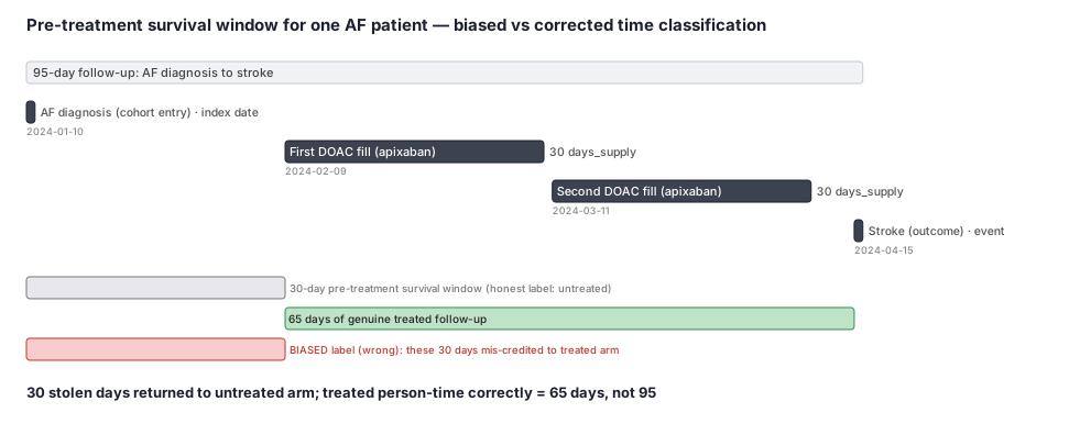
A researcher wants to know whether blood-thinners (DOACs) prevent stroke in patients newly diagnosed with atrial fibrillation (AF). She pulls claims data and finds every patient whose first AF diagnosis code appeared in 2024. She labels anyone who later filled a DOAC prescription as 'treated' and everyone else as 'untreated', then compares stroke rates from the AF diagnosis date forward. Patient 1001 was diagnosed on 2024-01-10 and picked up her first DOAC on 2024-02-09 — exactly 30 days later. The naive analysis credits those 30 days to the treated group. But a patient who suffers a fatal stroke on 2024-01-25 — before ever filling a prescription — is forced into the untreated group. The treated group never loses anyone in those first 30 days; the untreated group absorbs all early deaths. The treated group's stroke rate looks artificially low.

Dataset

Claims records for one patient showing the AF diagnosis date (cohort entry) and the first DOAC fill. No stroke occurred during the pre-treatment window; stroke happened on 2024-04-15.

Steps

• Count the days from AF diagnosis to the first DOAC fill: 2024-02-09 minus 2024-01-10 = 30 days. These 30 days are the pre-treatment survival window.

• Biased approach — mislabel the window: credit all 30 days to the 'treated' arm. Patient 1001 is recorded as treated from day 1. The treated arm gains 30 days of guaranteed stroke-free time it did not earn through the drug.

• Correct approach — label the window honestly: patient 1001 contributes 30 days as 'untreated' (days 0–29) and then switches to 'treated' on day 30 (the fill date) and contributes 65 more treated days until the stroke on day 95 (2024-04-15 minus 2024-01-10).

• Under the biased approach the treated arm's stroke-free person-time includes those 30 stolen days, pushing the hazard ratio below 1.0 even if the drug does nothing.

• Under the correct approach those 30 days are returned to the untreated column, and the hazard ratio moves toward the true value — in real statin and DOAC studies this correction has erased apparent benefits that turned out to be pure arithmetic artifacts.

Result

Label

Pre-treatment survival window = 30 days (2024-01-10 to 2024-02-08). Biased treated person-time from cohort entry = 95 days. Correct untreated person-time = 30 days; correct treated person-time = 65 days. Returning those 30 days to the untreated column is the entire correction.

Value

30

Timeline Spec

Title

Pre-treatment survival window for one AF patient — biased vs corrected time classification

Window

Start

2024-01-10

End

2024-04-15

Label

95-day follow-up: AF diagnosis to stroke

Events

• Label

  AF diagnosis (cohort entry)

  Start

  2024-01-10

  Length Days

  1

  Quantity

  index date

• Label

  First DOAC fill (apixaban)

  Start

  2024-02-09

  Length Days

  30

  Quantity

  30 days_supply

• Label

  Second DOAC fill (apixaban)

  Start

  2024-03-11

  Length Days

  30

  Quantity

  30 days_supply

• Label

  Stroke (outcome)

  Start

  2024-04-15

  Length Days

  1

  Quantity

  event

Spans

• Kind

  unexposed

  Start

  2024-01-10

  End

  2024-02-08

  Label

  30-day pre-treatment survival window (honest label: untreated)

• Kind

  exposed

  Start

  2024-02-09

  End

  2024-04-14

  Label

  65 days of genuine treated follow-up

• Kind

  gap

  Start

  2024-01-10

  End

  2024-02-08

  Label

  BIASED label (wrong): these 30 days mis-credited to treated arm

Result

Label

30 stolen days returned to untreated arm; treated person-time correctly = 65 days, not 95

Value

30

Caption

Patient 1001's timeline. The 30-day gap between AF diagnosis and first DOAC fill is the pre-treatment survival window. The biased analysis mislabels it as treated time (orange), manufacturing a stroke-free head start. The corrected analysis labels it as untreated time (blue) and starts the treated clock only at the fill date.

Alt Text

Horizontal timeline for patient 1001 running from 2024-01-10 to 2024-04-15. A 30-day span from cohort entry to the first DOAC fill is shaded blue and labeled 'pre-treatment survival window (untreated)' in the corrected analysis, and highlighted orange with an annotation 'wrongly credited to treated arm' in the biased analysis. From the first fill on 2024-02-09 to the stroke on 2024-04-15 a 65-day green span is labeled 'genuine treated follow-up'. A vertical marker at 2024-04-15 is labeled 'stroke (outcome event)'.

Runnable example

import pandas as pd
from lifelines import CoxTimeVaryingFitter

def build_time_varying(cohort: pd.DataFrame, rx: pd.DataFrame) -> pd.DataFrame:
    # First exposure fill per person; persons absent from rx never become exposed.
    first_fill = (rx.sort_values(["person_id", "fill_date"])
                    .groupby("person_id", as_index=False)["fill_date"].first()
                    .rename(columns={"fill_date": "fill_date"}))
    df = cohort.merge(first_fill, on="person_id", how="left")

    # Days from the early time zero (index_date) to each transition, on a single clock.
    df["t_exit"] = (df["exit_date"] - df["index_date"]).dt.days
    df["t_fill"] = (df["fill_date"] - df["index_date"]).dt.days
    # Exposure starting at/after exit contributes nothing exposed; clamp into [0, t_exit].
    df["t_fill"] = df["t_fill"].clip(lower=0, upper=df["t_exit"])

    rows = []
    for r in df.itertuples(index=False):
        exposed_ever = pd.notna(r.fill_date) and r.t_fill < r.t_exit
        if not exposed_ever:
            # Entire follow-up is unexposed (includes patients who exited before filling).
            rows.append((r.person_id, 0, r.t_exit, 0, r.event))
        else:
            # Unexposed interval [0, t_fill): never carries the event.
            rows.append((r.person_id, 0, r.t_fill, 0, 0))
            # Exposed interval [t_fill, t_exit): carries the event if one occurred.
            rows.append((r.person_id, r.t_fill, r.t_exit, 1, r.event))
    out = pd.DataFrame(rows, columns=["person_id", "start", "stop", "exposed", "event"])
    return out[out["stop"] > out["start"]]

tv = build_time_varying(cohort, rx)
ctv = CoxTimeVaryingFitter()
ctv.fit(tv, id_col="person_id", event_col="event",
        start_col="start", stop_col="stop")
ctv.print_summary()  # HR for time-varying 'exposed' is immune to immortal time bias

library(data.table)
library(survival)

build_and_fit <- function(cohort, rx) {
  setDT(cohort); setDT(rx)
  setorder(rx, person_id, fill_date)
  first_fill <- rx[, .(fill_date = fill_date[1L]), by = person_id]
  d <- merge(cohort, first_fill, by = "person_id", all.x = TRUE)

  # Single clock in days from the early time zero (index_date).
  d[, `:=`(t_exit = as.integer(exit_date - index_date),
           t_fill = as.integer(fill_date - index_date))]
  d[, t_fill := pmin(pmax(t_fill, 0L), t_exit)]   # clamp into [0, t_exit]

  # Base record: full follow-up, event at exit.
  base <- d[, .(person_id, t_exit, event)]
  base[, `:=`(tstart = 0L)]
  tv <- tmerge(base, base, id = person_id,
               death = event(t_exit, event))
  # Add the time-dependent exposure: switches to 1 at the fill date (NA = never exposed).
  tv <- tmerge(tv, d[!is.na(fill_date) & t_fill < t_exit],
               id = person_id, exposed = tdc(t_fill))
  tv$exposed[is.na(tv$exposed)] <- 0L

  coxph(Surv(tstart, tstop, death) ~ exposed, data = tv)
}

fit_tv <- build_and_fit(cohort, rx)
summary(fit_tv)  # exposed HR free of immortal time; contrast with naive ever/never coxph