Clone-Censor-Weight for Per-Protocol Target-Trial Emulation

In plain language

Clone-censor-weight (CCW) is a technique for comparing two treatment strategies using real-world data when everyone in the study could plausibly follow either strategy on day one. The trick is that each person is placed into both groups simultaneously by creating two copies called clones; each clone is followed over time and removed from its group the moment the real person's behavior diverges from that group's rule, and then a statistical weight is applied to compensate for those removals so the comparison stays fair. This lets researchers answer a per-protocol question: what would the outcome have been if patients actually stuck to their assigned strategy from start to finish?

Clone-censor-weight (CCW)

is the standard device for estimating the per-protocol effect of treatment strategies that two or more eligible patients could still satisfy at time zero but that diverge only later — the setting where a naive design has no clean way to assign an arm. Classic examples are sustained strategies ("initiate treatment within a grace period and stay on it" vs "never initiate"), duration strategies ("treat for 12 months" vs "treat for 6 months"), and threshold/dynamic strategies ("start when eGFR crosses X"). Because every eligible person is, at baseline, compatible with every strategy, CCW makes that compatibility explicit: it clones each person into one copy per strategy, follows each clone under its assigned rule, artificially censors a clone the instant its observed behavior departs from that rule, and then weights the surviving clone-time by the inverse probability of remaining uncensored so the censored clones are represented by similar still-adherent clones.

Core estimand distinction

CCW targets the observational analog of the per-protocol effect of a sustained strategy — what the cumulative incidence (or hazard) would have been had everyone followed the assigned strategy exactly. This is not the intention-to-treat (initiation) contrast, which an active-comparator new-user design with baseline propensity-score adjustment already estimates cleanly. It is also not the naive "as-treated" or "ever-exposed" contrast, which classifies person-time by post-baseline behavior and so re-imports immortal time, selection on adherence, and time-varying confounding. The cloning step exists precisely because the strategies are not distinguishable at t0: assigning the arm from baseline data alone (as one would in active-comparator new-user) is impossible for "start within 30 days and persist," so instead of choosing an arm we place each person in both arms and let the data censor the incompatible clone later. The inverse-probability-of-censoring weighting (IPCW) that follows is, mechanically, a marginal structural model fit on a cloned scaffold; CCW is best understood as an MSM whose person-time has been duplicated to encode strategy membership.

Pros, cons, and trade-offs

- vs naive as-treated / ever-exposed: CCW eliminates immortal-time bias (no person-time is counted before the deviation that defines non-adherence), selection bias from post-baseline arm assignment, and confounding by time-varying factors that drive both adherence and the outcome. Cost: it answers a hypothetical full-adherence question that can diverge from real-world adherence, and it requires a correctly specified IPCW model. Prefer CCW for any sustained/dynamic strategy where as-treated is the only alternative — as-treated is almost always biased here. - vs landmark analysis: Landmark conditions on survival and exposure status up to a fixed landmark time, discards everyone who had the event or deviated before it, and answers a question about the selected survivors. CCW clones everyone at baseline and recovers the full eligible population through weighting, so it avoids the survivor selection landmark builds in and accommodates grace periods naturally. Cost: heavier specification (two weighting models, weight diagnostics) and bootstrap inference. Prefer landmark only when the scientific question really is about a post-baseline conditioning set; otherwise CCW is the more defensible per-protocol estimator. - vs marginal structural models / g-methods without cloning: A standard MSM or the g-formula can estimate sustained-strategy effects directly without cloning. CCW's advantage is interpretability and protocol transparency — the cloning + censoring rules force you to write down the strategy, the grace period, and the deviation definition exactly as a trial protocol would, which is why regulators and reviewers favor it. Cost: the clone expansion multiplies the dataset, induces within-person correlation (requiring robust/bootstrap variance), and can be less statistically efficient than a well-specified g-formula. Prefer CCW when explicit protocol/estimand specification and auditability matter (regulatory submissions, head-to-head sustained strategies); consider plain g-methods or TMLE on the cloned data when efficiency or double robustness is the priority.

When to use

Sustained, duration, or dynamic strategies where (a) eligible patients satisfy every strategy at baseline, (b) divergence happens during follow-up (grace-period starts, persistence, biomarker-triggered initiation), and (c) you want the effect under full adherence. CCW is the per-protocol engine of most one-arm and head-to-head target-trial emulations of treatment strategies rather than point interventions.

When NOT to use — and when it is actively misleading

- The strategies are fully distinguishable at baseline (e.g., drug A initiator vs drug B initiator, both single point decisions). Then an active-comparator new-user design with IPTW is simpler, more efficient, and equally valid; cloning adds dataset size and variance for no gain. - Deviation is a collider / informed by the outcome process. If patients stop because of early toxicity or declining health that itself predicts the outcome, and those drivers are unmeasured, the IPCW "no unmeasured determinants of censoring" assumption fails and CCW is biased — frequently more convincingly biased than a crude analysis because the machinery lends false credibility. - The grace period is so short (or the strategy so demanding) that the eligible-and-still-adherent stratum collapses. A handful of persistently adherent clones near the end of follow-up receive enormous weights; effective sample size craters and the estimate becomes a high-variance artifact of a few people. - Competing risks differ by strategy and are ignored. In elderly claims cohorts, death competes with the event and may itself depend on the strategy; a cause-specific-hazard CCW that censors at the competing event answers a different (and often less policy-relevant) question than one targeting the subdistribution / cumulative incidence. Pre-specify which. - Adherence is unobservable in the data. In Medicare Advantage-only person-time, fills are not captured, so the deviation rule cannot fire correctly and clones are censored (or not) spuriously — restrict to fee-for-service / full-benefit person-time before applying CCW.

Data-source operational depth

- Claims (FFS / commercial): Treatment status over time is reconstructed from pharmacy fills (`fill_date` + `days_supply`, stitched into on-treatment episodes with a stockpiling/grace rule). Require continuous medical + pharmacy enrollment so a "no fill" gap is a true gap, not missingness. Failure modes: MA-only person-time lacks FFS pharmacy/medical claims, so the adherence/deviation rule misfires — exclude it; differential competing risks (death) by strategy in elderly cohorts bias a cause-specific CCW unless handled; immortal time sneaks back in if the grace period is treated as "guaranteed survival" rather than encoded as eligible-but-uncensored clone-time; 90-day mail-order and free samples distort `days_supply` and therefore the deviation timing. - EHR: Orders + administrations give finer "on-treatment" granularity and capture reasons for deviation (toxicity, response), which is invaluable for arguing the IPCW assumption — but visit-driven capture means a patient who leaves the system looks like a deviation/censoring event when they merely changed providers. Link to fills to confirm the patient actually started, and model loss to follow-up as a separate censoring process. - Registry: Structured start/stop dates and adjudicated outcomes support clean cloning and censoring rules and are common in embedded/registry-based emulations; weak for complete longitudinal drug exposure, so link to claims for the full fill history and to a death index to firm up the competing-risk handling. - Linked claims-EHR-vital records: The ideal substrate (EHR reasons-for-deviation + claims completeness + reliable mortality for competing risks), at the cost of linkage selection and reconciling order/fill/service-date discrepancies before time-zero and deviation timing are assigned.

Worked claims example

Question: does initiating a statin within 6 months of a first MI and persisting vs never initiating reduce 1-year all-cause mortality, in a commercial + Medicare fee-for-service database? (1) Eligibility: adults with an incident MI hospitalization, 365 days of continuous A/B/D (or commercial medical+pharmacy) enrollment before discharge, and no statin fill in that lookback. Time zero = discharge date. (2) Strategies: S1 = fill a statin within a 180-day grace period and remain covered thereafter; S0 = never fill a statin. (3) Cloning: each eligible person becomes two clones, one assigned S1 and one assigned S0, both starting at t0. (4) Artificial censoring: the S0 clone is censored on the first day a statin fill is observed; the S1 clone is censored at day 180 if no statin has been filled by then (failed the grace period) and, after a fill, on the first day the patient's covered supply lapses beyond a 30-day permissible gap (failed persistence). A clone that has the outcome before deviating is not censored — its event counts. (5) IPCW: fit a pooled logistic model per arm for the probability of remaining uncensored in each month given time-varying covariates (recent hospitalizations, cardiac procedures, comorbidity flags, prior adherence proxies) and baseline covariates; the stabilized weight for a clone-month is the cumulative product of those inverse probabilities. (6) Estimation: fit a weighted pooled logistic outcome model on the clone-months with a flexible function of time and a strategy indicator; convert the fitted discrete hazards into standardized 1-year cumulative-incidence curves and report the risk difference and risk ratio at 12 months. (7) Inference & diagnostics: nonparametric bootstrap over persons (resample whole persons, re-clone, refit weights and outcome model) for confidence intervals; report unique N vs expanded clone-months, the stabilized-weight distribution and effective sample size, and sensitivity analyses to the grace-period length (90 vs 180 vs 270 days), the permissible-gap rule, and weight truncation at the 1st/99th percentiles.

Interpreting the output

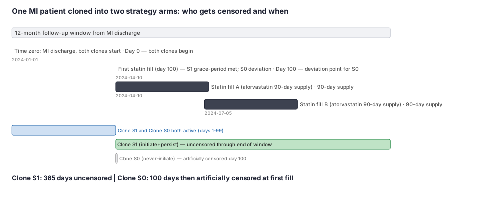
Using the worked example: Clone S1 (initiate-and-persist) contributes 365 uncensored days; Clone S0 (never-initiate) is artificially censored at day 100 when Maria fills her first statin. After IPCW reweighting across the full cohort, a per-protocol comparison yields — for illustration — HR = 0.74 (95% CI 0.61–0.90) for 1-year mortality.

Formal interpretation: The clone-censor-weight HR of 0.74 is the per-protocol effect of the initiate-and-persist strategy versus the never-initiate strategy — the causal effect that would be observed if all patients in the target population had adhered to their assigned strategy throughout follow-up. It is not an intent-to-treat estimate (which includes non-adherers) and does not apply to the as-treated population. The IPCW step is essential: without reweighting, patients who deviated (like Maria's Clone S0 at day 100) would be dropped, leaving a selected, healthier subgroup. The estimate is valid under two untestable conditions: no unmeasured confounding conditional on covariates entering the IPCW model, and correct specification of the censoring model. Confidence intervals must be obtained by cluster bootstrap over original patients — not over expanded clone-months — to respect the within-patient correlation introduced by cloning.

Practical interpretation: Patients who initiated a statin within 180 days and remained on it would, on average, have died at a 26% lower rate than those who never started — if the adherence assumptions and no-unmeasured-confounding conditions hold. The clone-censor-weight framework makes this "what if everyone had followed the strategy" question answerable from observational data without requiring treatment to have been randomized.

Worked example

Scenario

A researcher wants to know whether starting a statin within 180 days of a heart attack and staying on it reduces one-year mortality compared to never starting one. Using a claims database, every eligible patient is cloned into two copies at hospital discharge (day 0). Clone S1 is assigned to the initiate-and-persist strategy; Clone S0 is assigned to the never-initiate strategy. We follow one patient, Maria, to see exactly when and why each of her clones gets artificially censored.

Dataset

Maria's statin fill history after her MI discharge on 2024-01-01, as it would appear in a pharmacy claims table.

Steps

• At time zero (2024-01-01, Maria's discharge date), she is cloned: Clone S1 is assigned to the initiate-and-persist arm; Clone S0 is assigned to the never-initiate arm.

• Both clones begin follow-up on 2024-01-01. Neither has deviated yet, so both remain active.

• Maria fills atorvastatin on 2024-04-10, which is day 100 after discharge. This is within the 180-day grace period, so Clone S1 has met its initiation requirement and stays active.

• That same fill (2024-04-10) is the first statin observed in the data. Clone S0 is assigned to never initiate, so this fill is a deviation from S0's rule. Clone S0 is artificially censored on 2024-04-10 (day 100).

• Clone S1 continues follow-up. The 90-day fill covers through 2024-07-08. Maria refills on 2024-07-05, which is 3 days before the supply runs out, so there is no gap beyond 30 days. Persistence is maintained; Clone S1 stays active through the end of the 12-month window.

• Because Clone S0 was censored early, it only contributed 100 days of person-time to the never-initiate arm. To avoid systematically underrepresenting patients like Maria (those who eventually did start), the analyst fits an inverse-probability-of-censoring model and assigns a weight to the remaining S0 clones that resemble Maria's baseline profile.

Result

Clone S1 contributes 365 uncensored days under the initiate-and-persist strategy. Clone S0 contributes 100 days before artificial censoring at day 100 (2024-04-10). The per-protocol analysis weights Clone S0 records to account for this early removal, then compares 1-year mortality rates across both arms using those weights.

Timeline Spec

Title

One MI patient cloned into two strategy arms: who gets censored and when

Window

Start

2024-01-01

End

2024-12-31

Label

12-month follow-up window from MI discharge

Events

• Label

  Time zero: MI discharge, both clones start

  Start

  2024-01-01

  Quantity

  Day 0 — both clones begin

• Label

  First statin fill (day 100) — S1 grace-period met; S0 deviation

  Start

  2024-04-10

  Quantity

  Day 100 — deviation point for S0

• Label

  Statin fill A (atorvastatin 90-day supply)

  Start

  2024-04-10

  Length Days

  90

  Quantity

  90-day supply

• Label

  Statin fill B (atorvastatin 90-day supply)

  Start

  2024-07-05

  Length Days

  90

  Quantity

  90-day supply

Spans

• Kind

  followup

  Start

  2024-01-01

  End

  2024-04-09

  Label

  Clone S1 and Clone S0 both active (days 1-99)

• Kind

  exposed

  Start

  2024-04-10

  End

  2024-12-31

  Label

  Clone S1 (initiate+persist) — uncensored through end of window

• Kind

  unexposed

  Start

  2024-04-10

  End

  2024-04-10

  Label

  Clone S0 (never-initiate) — artificially censored day 100

Result

Label

Clone S1: 365 days uncensored | Clone S0: 100 days then artificially censored at first fill

Caption

Maria is cloned at time zero into two arms. Clone S1 (initiate and persist) remains active all year because she filled within the 180-day grace period and maintained continuous supply. Clone S0 (never initiate) is artificially censored on day 100 the moment the first fill appears. Inverse-probability-of-censoring weights compensate for the censored S0 person-time so the per-protocol comparison remains unbiased.

Alt Text

A timeline from 2024-01-01 to 2024-12-31 showing two parallel arms for one patient. Both arms are active from January through April 9. On April 10 (day 100), the S1 arm continues uncensored while the S0 arm ends with an artificial censoring marker. Two statin fill bars sit on the S1 arm: the first from April 10 through July 8, the second from July 5 through October 2, illustrating continuous coverage with a minor overlap.

Runnable example

import numpy as np
import pandas as pd
import statsmodels.formula.api as smf

GRACE_DAYS = 180          # window to initiate the statin and remain "adherent" to S1
GAP_DAYS = 30             # permissible gap before a persistence lapse counts as deviation
HORIZON_M = 12            # months of follow-up for the 1-year risk contrast

def build_person_periods(cohort, rx, outcome, fup_end):
    """One row per person-month from t0 to t0+HORIZON_M, with time-varying on-treatment + event flags."""
    rows = []
    rx_by = {p: g.sort_values("fill_date") for p, g in rx.groupby("person_id")}
    for r in cohort.itertuples(index=False):
        pid, t0 = r.person_id, r.t0
        ev = outcome.loc[outcome.person_id == pid, "event_date"]
        ev_date = ev.min() if len(ev) else pd.NaT
        adm = fup_end.loc[fup_end.person_id == pid, "fup_end_date"]
        adm_date = adm.min() if len(adm) else pd.NaT
        fills = rx_by.get(pid, pd.DataFrame(columns=["fill_date", "days_supply"]))
        # covered-day intervals stitched with stockpiling (carry-over of surplus supply)
        covered_until = t0 - pd.Timedelta(days=1)
        intervals = []
        for f in fills.itertuples(index=False):
            start = max(f.fill_date, covered_until + pd.Timedelta(days=1))
            covered_until = max(covered_until, f.fill_date) + pd.Timedelta(days=int(f.days_supply))
            intervals.append((start, covered_until))
        first_fill = fills["fill_date"].min() if len(fills) else pd.NaT
        for m in range(HORIZON_M):
            m_start = t0 + pd.Timedelta(days=30 * m)
            m_end = t0 + pd.Timedelta(days=30 * (m + 1)) - pd.Timedelta(days=1)
            if pd.notna(adm_date) and adm_date < m_start:
                break
            on_tx = any(s <= m_end and e + pd.Timedelta(days=GAP_DAYS) >= m_start for s, e in intervals)
            started_by = pd.notna(first_fill) and first_fill <= m_end
            event_m = int(pd.notna(ev_date) and m_start <= ev_date <= m_end)
            rows.append(dict(person_id=pid, month=m, on_tx=int(on_tx),
                             started_by=int(started_by),
                             days_since_t0=(m_start - t0).days, event=event_m))
            if event_m:
                break
    pp = pd.DataFrame(rows)
    return pp.merge(cohort, on="person_id", how="left")

def expand_and_censor(pp):
    """Duplicate each person-month into clone S1 and clone S0; set artificial censoring per the strategy."""
    out = []
    for strat in ("S1", "S0"):
        c = pp.copy()
        c["strategy"] = strat
        c["clone_id"] = c["person_id"].astype(str) + "_" + strat
        if strat == "S0":                       # never initiate -> censor at first treatment
            c["artif_cens"] = (c["on_tx"] == 1).astype(int)
        else:                                   # initiate within grace, then persist
            grace_fail = (c["days_since_t0"] > GRACE_DAYS) & (c["started_by"] == 0)
            persist_fail = (c["started_by"] == 1) & (c["on_tx"] == 0)
            c["artif_cens"] = (grace_fail | persist_fail).astype(int)
        out.append(c)
    x = pd.concat(out, ignore_index=True)
    # An event in a month overrides artificial censoring: the event is observed, not censored.
    x.loc[x["event"] == 1, "artif_cens"] = 0
    return x.sort_values(["clone_id", "month"])

def stabilized_ipcw(clones, tv_covs):
    """Pooled-logistic IPCW: P(uncensored this month). Stabilized weight = prod(num)/prod(denom)."""
    clones = clones.copy()
    clones["uncens"] = 1 - clones["artif_cens"]
    rhs_den = "bs(days_since_t0, df=4) + " + " + ".join(tv_covs)
    rhs_num = "bs(days_since_t0, df=4)"
    w = []
    for strat, g in clones.groupby("strategy"):
        den = smf.logit("uncens ~ " + rhs_den, data=g).fit(disp=0)
        num = smf.logit("uncens ~ " + rhs_num, data=g).fit(disp=0)
        g = g.assign(p_den=den.predict(g), p_num=num.predict(g))
        g = g.sort_values(["clone_id", "month"])
        g["sw"] = (g.groupby("clone_id")["p_num"].cumprod() /
                   g.groupby("clone_id")["p_den"].cumprod())
        w.append(g)
    out = pd.concat(w, ignore_index=True)
    out["sw"] = out["sw"].clip(upper=out["sw"].quantile(0.99))   # truncate extreme weights
    return out

def run_ccw(cohort, rx, outcome, fup_end, tv_covs=("on_tx",)):
    pp = build_person_periods(cohort, rx, outcome, fup_end)
    clones = expand_and_censor(pp)
    wdat = stabilized_ipcw(clones, list(tv_covs))
    # Weighted pooled-logistic outcome model (discrete-time hazard) on uncensored clone-months.
    m = smf.glm("event ~ strategy + bs(days_since_t0, df=4)",
                data=wdat[wdat["artif_cens"] == 0],
                family=__import__("statsmodels.api", fromlist=["families"]).families.Binomial(),
                freq_weights=wdat.loc[wdat["artif_cens"] == 0, "sw"]).fit()
    # Standardize: predict monthly hazard under each strategy, convert to 1-year cumulative incidence.
    risks = {}
    grid = wdat[["days_since_t0"]].drop_duplicates().sort_values("days_since_t0")
    for strat in ("S1", "S0"):
        g = grid.assign(strategy=strat)
        h = m.predict(g).values
        risks[strat] = 1 - np.prod(1 - h)
    return dict(model=m, risk_S1=risks["S1"], risk_S0=risks["S0"],
                risk_difference=risks["S1"] - risks["S0"])

library(data.table)
library(splines)

GRACE_DAYS <- 180L; GAP_DAYS <- 30L; HORIZON_M <- 12L

build_person_periods <- function(cohort, rx, outcome, fup_end) {
  setDT(cohort); setDT(rx); setDT(outcome); setDT(fup_end); setorder(rx, person_id, fill_date)
  out <- list()
  for (i in seq_len(nrow(cohort))) {
    pid <- cohort$person_id[i]; t0 <- cohort$t0[i]
    ev  <- min(outcome[person_id == pid, event_date],  Inf)
    adm <- min(fup_end[person_id == pid, fup_end_date], Inf)
    f   <- rx[person_id == pid]
    # stitch covered-day intervals with stockpiling carry-over
    covered_until <- t0 - 1L; iv <- list(); first_fill <- if (nrow(f)) min(f$fill_date) else as.Date(NA)
    if (nrow(f)) for (j in seq_len(nrow(f))) {
      start <- max(f$fill_date[j], covered_until + 1L)
      covered_until <- max(covered_until, f$fill_date[j]) + f$days_supply[j]
      iv[[length(iv) + 1L]] <- c(start, covered_until)
    }
    for (m in 0:(HORIZON_M - 1L)) {
      ms <- t0 + 30L * m; me <- t0 + 30L * (m + 1L) - 1L
      if (is.finite(adm) && adm < ms) break
      on_tx <- any(vapply(iv, function(z) z[1] <= me && z[2] + GAP_DAYS >= ms, logical(1)))
      started_by <- !is.na(first_fill) && first_fill <= me
      event_m <- as.integer(is.finite(ev) && ev >= ms && ev <= me)
      out[[length(out) + 1L]] <- data.table(person_id = pid, month = m,
        on_tx = as.integer(on_tx), started_by = as.integer(started_by),
        days_since_t0 = as.integer(ms - t0), event = event_m)
      if (event_m == 1L) break
    }
  }
  merge(rbindlist(out), cohort, by = "person_id")
}

expand_and_censor <- function(pp) {
  mk <- function(strat) {
    c <- copy(pp); c[, `:=`(strategy = strat, clone_id = paste0(person_id, "_", strat))]
    if (strat == "S0") c[, artif_cens := as.integer(on_tx == 1L)]
    else c[, artif_cens := as.integer((days_since_t0 > GRACE_DAYS & started_by == 0L) |
                                      (started_by == 1L & on_tx == 0L))]
    c
  }
  x <- rbindlist(list(mk("S1"), mk("S0")))
  x[event == 1L, artif_cens := 0L]          # observed events are not artificially censored
  setorder(x, clone_id, month); x[]
}

stabilized_ipcw <- function(clones, tv_covs = c("on_tx")) {
  clones[, uncens := 1L - artif_cens]
  fden <- as.formula(paste("uncens ~ bs(days_since_t0, df = 4) +", paste(tv_covs, collapse = " + ")))
  fnum <- uncens ~ bs(days_since_t0, df = 4)
  res <- clones[, {
    den <- glm(fden, data = .SD, family = binomial()); num <- glm(fnum, data = .SD, family = binomial())
    pd <- predict(den, .SD, type = "response"); pn <- predict(num, .SD, type = "response")
    ord <- order(clone_id, month)
    .SD[ord][, sw := ave(pn[ord], clone_id[ord], FUN = cumprod) /
                   ave(pd[ord], clone_id[ord], FUN = cumprod)][]
  }, by = strategy]
  res[, sw := pmin(sw, quantile(sw, 0.99))]      # truncate extreme weights
  res[]
}

run_ccw <- function(cohort, rx, outcome, fup_end, tv_covs = c("on_tx")) {
  pp <- build_person_periods(cohort, rx, outcome, fup_end)
  w  <- stabilized_ipcw(expand_and_censor(pp), tv_covs)
  fit <- glm(event ~ strategy + bs(days_since_t0, df = 4),
             data = w[artif_cens == 0L], family = binomial(), weights = w[artif_cens == 0L, sw])
  grid <- unique(w[, .(days_since_t0)])[order(days_since_t0)]
  risk <- sapply(c("S1", "S0"), function(s) {
    h <- predict(fit, cbind(grid, strategy = s), type = "response"); 1 - prod(1 - h)
  })
  list(fit = fit, risk_S1 = risk["S1"], risk_S0 = risk["S0"],
       risk_difference = unname(risk["S1"] - risk["S0"]))
}