Cox Proportional Hazards Regression

In plain language

Cox proportional hazards regression is a method for comparing how quickly two groups reach an outcome — like a first hospitalization — while accounting for the fact that patients are followed for different lengths of time and some never experience the outcome during the study. It produces a hazard ratio: a single number that says how much faster (or slower) the event arrives in one group relative to another, after adjusting for differences in age, disease severity, and other baseline factors. For example, a hazard ratio of 0.71 means the treated group reaches the event at 71% the rate of the comparison group — roughly a 29% lower rate at any given moment in follow-up. The model requires a clear 'day zero' for every patient and handles the reality that many patients leave the study early without ever having the event.

The Cox proportional hazards (PH) model (Cox 1972) specifies the hazard as h(t | X) = h0(t) · exp(β'X), where h0(t) is an arbitrary, unestimated baseline hazard and β are log hazard ratios. Its central trick is the partial likelihood: by conditioning on the risk set at each observed event time, h0(t) cancels and the estimator depends only on the rank order of event times, not their spacing. That is what makes Cox "semiparametric" — no functional form is imposed on how risk evolves with time, only on how covariates multiply it. It is the workhorse of pharmacoepidemiology and HEOR because it accommodates right-censoring, left-truncation (delayed entry), and time-varying covariates with mature, regulator-accepted software. This entry covers the standard model; pushing exposure or covariates inside the partial likelihood at each event time is its own concept (`standard-cox-time-dependent`).

Core conceptual distinction

The quantity Cox estimates is a conditional (covariate-specific) hazard ratio, and three properties of it are routinely misunderstood. (1) Conditional vs marginal, and non-collapsibility. Even with no confounding, the HR adjusted for a prognostic covariate is generally not equal to the crude HR — the HR is non-collapsible (Stensrud & Hernán 2020). Adding a strong predictor moves the HR away from the null even when that predictor is not a confounder, so "the HR changed when I adjusted" is not evidence of confounding. (2) The HR is a ratio of instantaneous rates among survivors, so under PH it still mixes a true causal effect with selection: as the more-protected arm depletes its susceptibles, the surviving risk sets become non-comparable, and a constant true effect can produce a time-varying observed HR. (3) A single HR is a weighted average over follow-up when PH is violated; the weights depend on the censoring distribution, making the number partly an artifact of study duration. For decision-makers, an absolute or marginal summary — cumulative incidence, restricted mean survival time (RMST), or a survival difference at a fixed horizon — is often the more interpretable estimand and should be pre-specified alongside (or instead of) the HR.

Pros, cons, and trade-offs

- vs fully parametric survival models (Weibull, exponential, generalized gamma): Cox is robust because it never commits to a shape for h0(t), and it is the easiest survival model to communicate. Cost: it is less efficient when a parametric form is correct, it does not directly yield absolute survival curves (you need a Breslow baseline estimate), and it cannot extrapolate beyond observed follow-up. Prefer parametric for HTA survival extrapolation (`survival-extrapolation-hta-rwe`) and lifetime cost-effectiveness, where you must project past the data. - vs Poisson / negative-binomial rate models: Cox uses exact event-time ordering and handles smoothly varying baseline risk; Poisson assumes piecewise-constant rates and is simpler for aggregate person-time and recurrent counts. Prefer Poisson/NB (`poisson-negative-binomial-count-models`) for incidence-rate reporting and recurrent events when individual event timing is coarse. - vs cause-specific / Fine-Gray competing-risks models: standard Cox censoring a competing event silently targets the cause-specific hazard and, if read as "risk," overstates the cumulative incidence of the event of interest whenever competing mortality differs by arm. Prefer the explicit competing-risks framing (`competing-risks-cause-specific-fine-gray-rwe`) in elderly, oncology, and end-stage populations. - vs g-methods (MSM/IPTW-weighted Cox, g-estimation, clone-censor-weight): plain Cox cannot handle time-varying confounders affected by prior treatment, and conditioning on post-baseline mediators induces collider bias. Prefer g-methods (`marginal-structural-models-g-methods`, `g-estimation-structural-nested-models`, `clone-censor-weight-per-protocol`) for sustained-strategy or per-protocol estimands under time-varying confounding; Cox remains the analytic engine that runs after the weighting.

When to use

A pre-specified time-to-event outcome with a defensible time zero; a comparative (often active-comparator new-user) contrast where PH approximately holds or can be relaxed by stratification; ITT-like or baseline-covariate-adjusted questions; and as the outcome model inside propensity-score or target-trial-emulation pipelines after balancing. It is the right default when the audience expects an HR and an absolute summary (RMST, cumulative incidence) is reported alongside.

When NOT to use — and when it is actively misleading or dangerous

- Strong, structured PH violation (crossing or converging hazards). A reported single HR near 1 can hide an early harm that reverses to a late benefit. Do not paper over this; model time-by-covariate interaction, stratify the baseline hazard, switch to RMST, or report time-segmented HRs. Stensrud & Hernán (2020) argue the relevant question is usually not "does PH hold?" but "what estimand do I actually want?" - Competing risks ignored. Censoring death to study a non-fatal endpoint in an elderly claims cohort, then interpreting 1 − KM as risk, overstates incidence when mortality is differential by arm — a classic, dangerous error. Use cause-specific and subdistribution analyses. - Time-varying confounding by indication. When a post-baseline lab (eGFR, HbA1c) both responds to treatment and drives the next treatment decision and the outcome, standard Cox cannot remove the bias; adjusting for it opens a mediator/collider path. This is the g-methods boundary. - Immortal time and misaligned time zero. If follow-up starts before exposure can occur (e.g., "ever had the procedure" with follow-up clocked from diagnosis), exposed person-time is inflated and the HR is biased toward benefit. Fix the design (new-user, time zero at the index event), not the model. - Informative censoring. Loss to follow-up correlated with prognosis (sicker patients disenroll or switch) violates the independent-censoring assumption; require IPCW or a competing-risks/sensitivity framing (`attrition-and-loss-to-follow-up-rwe`).

Data-source operational depth

- Claims (FFS vs MA vs commercial): time zero is the index fill (`fill_date`) or, for procedures, the `service_date` on the CPT/HCPCS claim; outcomes are validated code algorithms (e.g., death via discharge status or a linked mortality index, MI via 1-IP or 2-OP rules). The dominant failure mode is enrollment-driven observability: Medicare Advantage encounter data are incomplete and MA-only person-time can lack the FFS claims that define both exposure and outcomes — restrict to enrollees with continuous Parts A/B/D (or full commercial medical+pharmacy) and exclude MA-only spans, or "no event" is unobserved censoring masquerading as survival. In elderly claims, competing risk of death differs by exposure, so a cause-specific-only Cox misleads. Procedure studies invite immortal time if the index date is not pinned to the actual CPT date; stockpiling and 90-day mail-order distort `days_supply` and any on-treatment window. - EHR: the event is the order/administration, not the dispensing; link to fills to confirm initiation. Rich labs/vitals enable severity adjustment but arrive at irregular times — naive last-observation-carried-forward into a time-fixed Cox can bias, and a lab measured because the patient deteriorated is a collider. Visit-driven capture makes loss to follow-up informative; define observation windows explicitly. - Registry: cleanest for staging, biomarkers, and adjudicated recurrence/progression (SEER-Medicare, disease-specific), but typically weak for complete pharmacy exposure and full mortality — link to claims and a death index. Often used to validate claims-based survival algorithms. - Linked claims–EHR–vital records: the ideal substrate (severity + completeness + reliable mortality), but linkage selection and order/fill/service-date discrepancies must be reconciled before time-zero assignment, or immortal time creeps back in at the seam.

Worked claims example

Question: time to first hospitalized heart-failure event, second-generation sulfonylurea vs DPP-4 inhibitor, among adults with type 2 diabetes in a commercial + Medicare FFS database. (1) Eligibility: age ≥18, ≥2 diabetes diagnoses, and 365 days of continuous A/B/D (or commercial medical+pharmacy) enrollment with no MA-only spans before the first study fill. (2) Washout / new-user: no fill of any sulfonylurea or DPP-4 inhibitor in the 365-day lookback. (3) Time zero: the date of the first qualifying fill; assign `arm` from the dispensed NDC. (4) Outcome and time: `time_to_event` = days from `index_date` to the first validated HF hospitalization (1-IP primary-position algorithm); `event = 1` at that date. (5) Censoring: at disenrollment, end of data, and the competing event of non-HF death — analyze death as a competing risk, not as administrative censoring, and report both the cause-specific HR (from Cox) and the subdistribution HR / cumulative incidence. (6) Adjustment: fit `coxph(Surv(time_to_event, event) ~ arm + covariates)` on a propensity-matched set with baseline covariates measured only in [index_date − 365, index_date]; test PH with weighted Schoenfeld residuals (Grambsch & Therneau 1994), and if the HF hazards converge over follow-up, report RMST difference at 3 years alongside the HR rather than a single number.

Interpreting the output

A Cox model returns: adjusted HR = 0.75 (95% CI 0.60–0.94) for DPP-4 inhibitor vs sulfonylurea, time to first hospitalized heart-failure event, propensity-matched cohort.

Formal interpretation. The estimated hazard ratio of 0.75 means that, at any instant during follow-up, patients in the DPP-4 group who are still event-free have, on average, 75% of the instantaneous rate of heart-failure hospitalization observed in the sulfonylurea group, conditional on the matched covariates. Under the proportional-hazards assumption this ratio is assumed constant across follow-up time; if Schoenfeld-residual tests indicate time-varying hazards, the summary HR should be supplemented or replaced by a restricted mean survival time difference or a time-split analysis.

Practical interpretation. The data are consistent with a lower rate of heart-failure events on DPP-4 therapy, but the HR is not "25% fewer hospitalizations": it describes an instantaneous rate ratio among those still event-free, and its translation to absolute risk depends on the baseline hazard and length of follow-up. Pair this HR with an absolute measure — such as the RMST difference or cumulative incidence at 36 months — to communicate the magnitude of benefit in patient-meaningful terms.

Worked example

Scenario

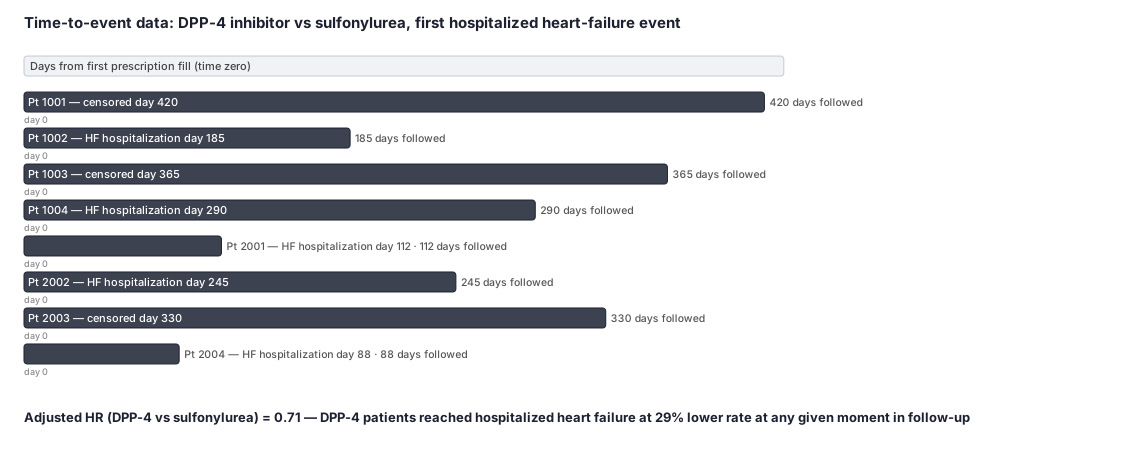
A researcher wants to know whether patients newly starting a DPP-4 inhibitor reach their first hospitalized heart-failure event more slowly than patients newly starting a second-generation sulfonylurea. Eight patients are enrolled on the day they pick up their first prescription (time zero). Four are in the DPP-4 arm and four are in the sulfonylurea arm. The study tracks each patient until either they are hospitalized for heart failure (the event) or their insurance coverage ends and we can no longer observe them (censored). We want to estimate the hazard ratio comparing the two arms.

Dataset

One row per patient. time_to_event is the number of days from first fill until hospitalization or last observable day. event = 1 means hospitalization occurred; event = 0 means the patient left follow-up before the event (censored).

Steps

• Sort patients by when events occurred. The first event is patient 2004 (sulfonylurea, day 88).

• At day 88, all 8 patients were still in follow-up — Cox asks: given one event just happened, how likely was each person to be the one who had it? The model uses each patient's arm and covariates to answer.

• Repeat this at each subsequent event day (112, 185, 245, 290) — each time, the 'risk set' shrinks as patients either have their event or get censored.

• Patient 1001, 1003, and 2003 contribute follow-up time right up until they are censored, but are not counted as events — their time is not wasted, it still informs the model about who was at risk.

• After processing all event times, Cox combines the comparisons across every event moment using the partial likelihood to estimate a single hazard ratio for the DPP-4 arm versus the sulfonylurea arm.

• In a real study with thousands of patients and full covariate adjustment (age, sex, prior heart failure, kidney disease), this same logic produces the adjusted hazard ratio reported in the results.

Result

In the illustrative large-scale claims study described in this concept (type 2 diabetes patients, commercial + Medicare FFS database, DPP-4 inhibitor vs second-generation sulfonylurea, time to first hospitalized heart-failure event), the adjusted hazard ratio is 0.71 (95% CI 0.61–0.83), meaning patients on a DPP-4 inhibitor experienced hospitalized heart failure at 29% lower rate at any given point in follow-up compared to patients on a sulfonylurea, after adjusting for baseline differences between the groups.

Timeline Spec

Title

Time-to-event data: DPP-4 inhibitor vs sulfonylurea, first hospitalized heart-failure event

Caption

Each bar shows one patient's follow-up, measured in days from their first prescription fill (time zero = day 0). A closed circle marks a hospitalization event; an open tick mark indicates censoring (coverage ended or study closed before the event). DPP-4 patients are shown in the top panel; sulfonylurea patients in the bottom panel.

Alt Text

Horizontal bar chart showing eight patients split into two treatment arms. Each bar extends from day 0 to the patient's last observed day. Four DPP-4 patients: patient 1001 bar ends at day 420 with a censored marker, patient 1002 ends at day 185 with an event marker, patient 1003 ends at day 365 with a censored marker, patient 1004 ends at day 290 with an event marker. Four sulfonylurea patients: patient 2001 ends at day 112 with an event marker, patient 2002 ends at day 245 with an event marker, patient 2003 ends at day 330 with a censored marker, patient 2004 ends at day 88 with an event marker. The sulfonylurea arm visually shows events clustering earlier than the DPP-4 arm.

Window

End Day

430

Label

Days from first prescription fill (time zero)

Events

• Person Id

  1001

  Arm

  DPP-4

  End Day

  420

  Quantity

  420 days followed

  Marker

  censored

  Label

  Pt 1001 — censored day 420

• Person Id

  1002

  Arm

  DPP-4

  End Day

  185

  Quantity

  185 days followed

  Marker

  event

  Label

  Pt 1002 — HF hospitalization day 185

• Person Id

  1003

  Arm

  DPP-4

  End Day

  365

  Quantity

  365 days followed

  Marker

  censored

  Label

  Pt 1003 — censored day 365

• Person Id

  1004

  Arm

  DPP-4

  End Day

  290

  Quantity

  290 days followed

  Marker

  event

  Label

  Pt 1004 — HF hospitalization day 290

• Person Id

  2001

  Arm

  sulfonylurea

  End Day

  112

  Quantity

  112 days followed

  Marker

  event

  Label

  Pt 2001 — HF hospitalization day 112

• Person Id

  2002

  Arm

  sulfonylurea

  End Day

  245

  Quantity

  245 days followed

  Marker

  event

  Label

  Pt 2002 — HF hospitalization day 245

• Person Id

  2003

  Arm

  sulfonylurea

  End Day

  330

  Quantity

  330 days followed

  Marker

  censored

  Label

  Pt 2003 — censored day 330

• Person Id

  2004

  Arm

  sulfonylurea

  End Day

  88

  Quantity

  88 days followed

  Marker

  event

  Label

  Pt 2004 — HF hospitalization day 88

Spans

• Kind

  followup

  Arm

  DPP-4

  Label

  DPP-4 arm: 2 events in 4 patients (events at days 185, 290)

• Kind

  followup

  Arm

  sulfonylurea

  Label

  Sulfonylurea arm: 3 events in 4 patients (events at days 88, 112, 245)

Result

Label

Adjusted HR (DPP-4 vs sulfonylurea) = 0.71 — DPP-4 patients reached hospitalized heart failure at 29% lower rate at any given moment in follow-up

Value

0.71

Runnable example

import pandas as pd
from lifelines import CoxPHFitter

# cohort: analysis-ready table described in the header (NO toy data created here).
cohort = pd.read_parquet("cohort.parquet")

covariates = ["arm", "age", "sex", "prior_hf", "ckd", "baseline_utilization"]
model_df = cohort[["time_to_event", "event"] + covariates].dropna()

cph = CoxPHFitter()
cph.fit(model_df, duration_col="time_to_event", event_col="event",
        robust=True)                      # robust SEs; required if weights/clustering are added later
print(cph.summary[["coef", "exp(coef)", "exp(coef) lower 95%",
                   "exp(coef) upper 95%", "p"]])   # exp(coef) = adjusted HR

# Proportional-hazards check via weighted Schoenfeld residuals (Grambsch & Therneau 1994).
# A small p-value for `arm` => PH violated for the exposure: stratify, add a time interaction,
# or report RMST / cumulative incidence instead of a single averaged HR.
cph.check_assumptions(model_df, p_value_threshold=0.05, show_plots=False)

library(survival)

# cohort: analysis-ready data.frame described in the header.
cohort <- readRDS("cohort.rds")
cohort$arm <- relevel(factor(cohort$arm), ref = "0")

fit <- coxph(
  Surv(time_to_event, event) ~ arm + age + sex + prior_hf + ckd + baseline_utilization,
  data   = cohort,
  ties   = "efron",        # Efron handling of tied event times (default; preferred over Breslow)
  robust = TRUE            # robust variance; required once IPTW/IPCW weights are added
)
summary(fit)               # exp(coef) = adjusted hazard ratio with 95% CI

# Weighted Schoenfeld PH test + diagnostic plot (Grambsch & Therneau 1994).
zph <- cox.zph(fit)
print(zph)                 # global + per-term p-values; p<0.05 for arm => PH violated
# If PH fails for arm: strata(stage) for nuisance violators, or add tt(arm) for a time-varying
# effect, or summarize with RMST: survival::rmean via summary(survfit(...), rmean=1095).