Cox Regression with Time-Dependent Covariates

In plain language

A time-dependent Cox model is a survival analysis tool that tracks whether a patient is currently on a treatment at each moment of follow-up, rather than labeling them as a treated person for the entire study period. It splits each patient's follow-up into timed segments and asks, at any given day when an outcome event happens, who else was still being watched and what was their treatment status right then. This approach correctly handles the fact that a patient who starts a drug on day 90 of a study should not have their first 89 days counted as drug-exposed time. Without this correction, the pre-drug days get credited to the treatment group, creating a form of bias called immortal time bias that makes the drug look better than it is.

A time-dependent (time-varying) Cox model generalizes the standard proportional-hazards model by letting a covariate `x(t)` change value during follow-up. Mechanically, each subject's follow-up is split into multiple `(start, stop]` intervals — the counting-process (Andersen–Gill) data layout — and at every event time the partial likelihood compares the covariate value of the person who failed against the current covariate values of everyone still at risk. The hazard is `h(t | x(t)) = h0(t) * exp(beta' x(t))`, and `exp(beta)` is the hazard ratio per unit of the covariate as it is at time t. This is the correct way to model a status that switches on during follow-up (started a drug, was hospitalized, crossed a lab threshold, accrued cumulative dose) without committing the cardinal sin of using a future value to classify present person-time.

Core conceptual distinction

. The decision that does the work is when person-time is allowed to count toward an exposure group. A naive time-fixed analysis assigns a subject to the "exposed" group for their entire follow-up because they were exposed at some point, which credits the exposed group with person-time that was lived before exposure occurred — immortal time / guarantee-time bias, because to become exposed the subject had to survive event-free until the exposure happened. A time-dependent covariate fixes this: the subject contributes unexposed person-time from time zero until the moment of exposure, then exposed person-time thereafter, and the exposure indicator is 0 then 1 across the split intervals. The estimand is a hazard ratio comparing the instantaneous hazard under the covariate value held at each instant — an internal, association-style contrast. Critically, this is NOT a causal contrast of treatment strategies: when the time-varying exposure is affected by, and itself affects, time-varying confounders (e.g., disease severity drives both treatment switching and the outcome), standard time-dependent Cox is biased no matter how you condition, because conditioning on a post-baseline confounder that is also a mediator opens a collider path. The fix for that is a marginal structural model (IPTW-weighted pooled logistic / Cox) or g-estimation — not a richer time-dependent Cox.

Pros, cons, and trade-offs

- vs naive baseline-only ("ever exposed") Cox: time-dependent coding removes immortal-time bias and correctly aligns exposed person-time with exposed status. Cost: more programming, a counting-process dataset, and a model whose HR is harder to communicate (it is per-instant, not "over the study"). Prefer time-dependent whenever exposure status, dose, or a covariate genuinely changes after time zero and you are not estimating a strategy contrast. - vs landmark analysis: landmarking sidesteps immortal time by fixing exposure status at a pre-specified landmark time and analyzing only survivors to that point — simpler, robust, and avoids the post-baseline-confounding trap, but discards early events and answers a conditional question (survivors to the landmark). Prefer landmarking for a single one-way status change and a clean clinical message; prefer time-dependent Cox for repeatedly changing exposures, cumulative dose, or when you cannot afford to drop pre-landmark events. - vs marginal structural models / g-methods: when the time-varying exposure has time-varying confounders that are also on the causal pathway (confounder affected by prior treatment), time-dependent Cox is structurally biased and an MSM with inverse-probability-of-treatment weights (or g-estimation) is required. Prefer plain time-dependent Cox only when later covariates are not affected by earlier exposure; otherwise it is actively misleading. See marginal-structural-models-g-methods. - vs Fine–Gray / cause-specific competing-risks models: orthogonal concern — if a competing event (e.g., non-outcome death) precludes the event of interest, the time-dependent Cox should be specified as cause-specific, and absolute-risk statements need a cumulative-incidence (Fine–Gray) companion. See competing-risks-cause-specific-fine-gray-rwe.

When to use

. A covariate or exposure that switches value during follow-up (new medication start, hospitalization episode, time-updated lab/biomarker, cumulative dose, on/off treatment windows); recurrent-event or multi-state follow-up modeled in the Andersen–Gill counting-process framework; any analysis where a naive "ever-exposed" classification would manufacture immortal time. It is the default engine for time-updated exposures when there is no feedback between exposure and later confounders.

When NOT to use — and when it is actively misleading or dangerous

. - Time-varying confounding affected by prior treatment. This is the headline failure. If a confounder (CD4, eGFR, disease activity) responds to earlier exposure and also predicts later exposure and the outcome, conditioning on it in a time-dependent Cox biases the effect (collider/over-adjustment) while omitting it leaves residual confounding — there is no safe option. Use an MSM/g-methods. Mistaking this for "I just need more covariates" is the dangerous error. - Using a covariate value not yet observed at time t. Carrying a final or peak value backward, or coding exposure as 1 for person-time before the exposure date, silently re-introduces immortal-time/guarantee-time bias — the very bias the method exists to prevent. Every interval's covariate must be knowable from data available strictly at `start`. - A defined treatment strategy is the question (e.g., "initiate and stay on drug A vs B"). That is a sustained-strategy estimand for clone-censor-weight or an MSM, not an instantaneous time-dependent HR. - Reverse causation / the covariate is part of the outcome process. A lab that moves because the event is imminent (e.g., falling albumin in the days before death) will absorb the effect; the HR is then descriptive, not causal. - Proportional hazards is violated for the time-dependent term (its effect changes over time); then add an explicit covariate-by-time interaction or move to RMST/flexible models rather than reporting a single misleading HR.

Data-source operational depth

. - Claims (FFS vs MA): the time-varying exposure is built from pharmacy `fill_date` + `days_supply` (on-treatment episodes with stockpiling and grace rules) or from inpatient/procedure dates. The interval split must use the claim/service date, never the paid/adjudication date, or exposure onset is shifted by months of lag. Failure mode: Medicare Advantage enrollees lack fee-for-service claims, so on/off-drug and hospitalization intervals are unobservable — MA-only person-time masquerades as "unexposed," biasing the time-dependent indicator; restrict to A/B/D FFS (or commercial with pharmacy benefit) and exclude MA-only spans rather than treating them as exposure-free. Same-day duplicate/reversed claims and bundled services create spurious zero-length or overlapping intervals — collapse them before splitting. Plan switching fragments enrollment; left-truncated person-time (enrollment starts mid-history) must enter via `start` > 0, not at 0. - EHR: time-updated labs/vitals arrive at irregular, encounter-driven times; between measurements you must choose a carry-forward (last-observation-carried-forward) window and cap it, because a value carried for 18 months is fiction. Visit-driven capture means sicker patients are measured more often — informative observation that can bias a measurement-triggered exposure. External care leakage (treatment received outside the system) makes the on/off-exposure indicator wrong; prefer linkage to dispensing. - Registry: strong for adjudicated time-stamped clinical events (stage change, transplant date) but typically sparse between scheduled visits; reconcile registry event dates with claims/EHR before splitting, and treat between-visit gaps as genuinely unobserved. - Linked claims–EHR–vital records: the ideal substrate (EHR labs for the time-varying covariate, claims for complete drug/hospitalization episodes, death index for the outcome), but order/fill/service-date discrepancies across sources must be reconciled so each interval's covariate is anchored to a single, defensible clock — otherwise overlapping intervals from different sources double-count person-time.

Worked claims example

Question: does current statin exposure (time-varying on/off) change the hazard of incident myocardial infarction among adults with type 2 diabetes in a commercial + Medicare FFS database? (1) Cohort & time zero: age ≥18, ≥2 diabetes diagnoses, ≥365 days continuous A/B/D (or commercial medical+pharmacy) enrollment before time zero; time zero = first diabetes-qualifying date after enrollment; exclude MA-only person-time. (2) Outcome: first validated MI (e.g., 1 inpatient primary-position MI claim), date = service date. (3) Build statin episodes from `fill_date` + `days_supply`, stitching overlapping fills (stockpiling, cap at, say, 90 days) and bridging gaps ≤30 days (grace period); an MI's risk at a given day is classified by whether that day falls inside an on-statin episode. (4) Split each person's follow-up at every episode start/stop into `(start, stop]` intervals, set `statin_on` = 0/1 per interval, and set the event flag = 1 only on the interval whose `stop` is the MI date. (5) Right-censor at disenrollment, death, end of data; left-truncate any person-time before continuous enrollment via positive `start`. (6) Fit a Cox model on the counting-process data with `statin_on` as a time-dependent covariate plus baseline confounders (and time-updated confounders only if they are NOT affected by prior statin use — otherwise switch to an MSM). (7) Check PH for `statin_on` via scaled Schoenfeld residuals; if violated, add a `statin_on * log(t)` interaction. The contrast is the hazard of MI while currently on statin vs currently off, with each day of person-time credited to the status truly held that day — no immortal time.

Interpreting the output

A time-dependent Cox model of statin use and myocardial infarction returns: HR = 0.82 (95% CI 0.68–0.98) for current statin use vs current non-use, counting-process layout.

Formal interpretation. The estimated HR of 0.82 means that, at each instant of follow-up, a patient currently on statin has, on average, 82% of the instantaneous MI rate of an otherwise similar patient currently not on statin, among those still event-free. Because person-time is classified by actual statin status on each day — using a (start, stop, event) counting-process layout — days before the first fill contribute to unexposed person-time even for patients who later initiate, eliminating the immortal-time that inflates apparent benefit in naive time-fixed analyses. The PH assumption implies this ratio does not change with time; if the effect is plausibly early-versus-late, a time-split or log(t) interaction should be checked.

Practical interpretation. The HR captures "currently on" vs "currently off" treatment, not "ever-treated" vs "never-treated." This distinction matters when adherence is variable: partial users contribute both on- and off-treatment person-time, diluting the contrast toward the null. Report both the HR and a cumulative incidence difference at a fixed horizon to convey absolute benefit alongside the relative rate estimate.

Worked example

Scenario

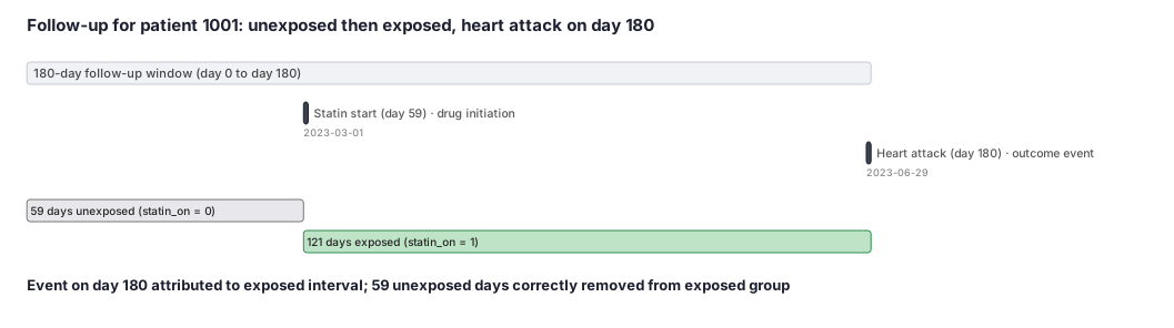
A researcher wants to know whether being currently on a statin reduces the rate of heart attack among adults with type 2 diabetes. Patient 1001 enters the study on 2023-01-01 without a statin prescription. She fills her first statin on day 60 (2023-03-01). She has a heart attack on day 180 (2023-06-29). The key question for the data analyst is: how should her 180 days of follow-up be divided between unexposed time (no statin) and exposed time (on statin)?

Dataset

Counting-process table for patient 1001 after splitting her follow-up at her statin start date. Each row is one interval; the exposure indicator reflects her actual status during that stretch of time.

Steps

• Patient 1001 enters the study at day 0 with no statin; statin_on is 0 for this first interval.

• On day 59, she fills her first statin prescription, so her follow-up is split into a new interval starting at day 59 where statin_on flips to 1.

• Her heart attack occurs on day 180, so the second interval ends at day 180 and the event flag is set to 1 on that final row.

• In the model, days 0-59 (59 days) contribute to the unexposed risk set and days 59-180 (121 days) contribute to the exposed risk set.

• If instead we had coded statin_on = 1 for all 180 days (naive ever-exposed approach), those first 59 event-free days would have been falsely credited to the statin group, inflating the apparent benefit of the drug.

Result

Unexposed person-time = 59 days (statin_on = 0); exposed person-time = 121 days (statin_on = 1); event attributed to the exposed interval. The hazard ratio for statin_on produced by the Cox model reflects the instantaneous rate of heart attack while currently on statin versus currently off statin, with no immortal time in the calculation.

Timeline Spec

Title

Follow-up for patient 1001: unexposed then exposed, heart attack on day 180

Window

Start

2023-01-01

End

2023-06-29

Label

180-day follow-up window (day 0 to day 180)

Events

• Label

  Statin start (day 59)

  Start

  2023-03-01

  Length Days

  1

  Quantity

  drug initiation

• Label

  Heart attack (day 180)

  Start

  2023-06-29

  Length Days

  1

  Quantity

  outcome event

Spans

• Kind

  unexposed

  Start

  2023-01-01

  End

  2023-02-28

  Label

  59 days unexposed (statin_on = 0)

• Kind

  exposed

  Start

  2023-03-01

  End

  2023-06-29

  Label

  121 days exposed (statin_on = 1)

Result

Label

Event on day 180 attributed to exposed interval; 59 unexposed days correctly removed from exposed group

Caption

Patient 1001 is unexposed for her first 59 days (no statin), then exposed from day 59 onward when she starts the drug. The time-dependent Cox model splits her follow-up at the drug start date so that each day is credited to the status she actually held. A naive ever-exposed analysis would have counted all 180 days as exposed, giving the statin credit for 59 event-free days it had nothing to do with.

Alt Text

Horizontal timeline from January 1 to June 29, 2023. A gray bar labeled 59 days unexposed spans January 1 through February 28. A green bar labeled 121 days exposed spans March 1 through June 29. A vertical marker on March 1 is labeled statin start day 59. A vertical marker on June 29 is labeled heart attack day 180.

Runnable example

import pandas as pd
from lifelines import CoxTimeVaryingFitter
from lifelines.statistics import proportional_hazard_test

# df is the counting-process table described in the header (one row per person-interval).
# Sanity check: intervals are well-formed and non-overlapping within person.
assert (df["t_stop"] > df["t_start"]).all(), "each interval needs t_stop > t_start"

ctv = CoxTimeVaryingFitter(penalizer=0.0)
ctv.fit(
    df,
    id_col="person_id",
    start_col="t_start",
    stop_col="t_stop",
    event_col="event",
    # statin_on enters at the value it holds in each interval -> time-dependent HR
    formula="statin_on + age + female + prior_cvd",
)
ctv.print_summary()  # exp(coef) for statin_on = HR of MI while currently on vs off statin

# Proportional-hazards check for the time-dependent term via scaled Schoenfeld residuals.
# If statin_on violates PH, refit with a step (Heaviside) or statin_on:log(t) interaction.
ph = proportional_hazard_test(ctv, df, time_transform="log")
print(ph.summary)

library(survival)

# Follow-up time in days from time zero; left truncation handled by tstart of the first interval.
base$fu_days   <- as.numeric(base$exit_date - base$time_zero)
statin$start_d <- as.numeric(statin$episode_start - base$time_zero[match(statin$person_id, base$person_id)])
statin$stop_d  <- as.numeric(statin$episode_end   - base$time_zero[match(statin$person_id, base$person_id)])

# Build the counting-process dataset: split at episode boundaries, carry the event to the final interval.
cp <- tmerge(base, base, id = person_id,
             mi = event(fu_days, event))
cp <- tmerge(cp, statin, id = person_id,
             statin_on = tdc(start_d))        # 1 from each episode start onward within the episode span

fit <- coxph(Surv(tstart, tstop, mi) ~ statin_on + age + female + prior_cvd,
             data = cp, id = person_id, ties = "efron")
summary(fit)                                  # exp(coef) for statin_on = current-exposure HR

# Proportional-hazards diagnostic on the time-dependent term (scaled Schoenfeld residuals).
cox.zph(fit)