Recurrent Events Analysis

In plain language

Recurrent events analysis counts every time an event happens to a patient — not just the first time — so you get the full picture of how often a disease flares up over a follow-up period. A patient with COPD may land in the hospital three times in one year; a method that only looks at the first hospitalization throws away two-thirds of the signal and may miss a drug that cuts the repeat rate in half. These methods track each patient from their start date, note every qualifying event in order, and then estimate an event rate or a cumulative event count for the whole group. The main honest limitation is that death can stop events from occurring, so a drug that keeps very sick patients alive longer may appear to cause more events in a naive analysis.

Recurrent-event outcomes

are events that a single patient can experience more than once over follow-up: COPD/asthma exacerbations, heart-failure hospitalizations, sickle-cell pain crises, infections under immunosuppression, severe hypoglycemia, falls, seizures, and most healthcare-resource-utilization (HCRU) endpoints. The naive habit of analyzing only time to first event throws away the majority of the information and, more importantly, answers a different question than payers and clinicians are asking. A drug that does not delay the first exacerbation but halves the long-run exacerbation rate will look null in a first-event Cox model and clearly beneficial in a recurrent-event model. The choice of method is therefore an estimand decision, not a software preference.

Core estimand distinction

Recurrent-event analyses split into three estimand families that are NOT interchangeable. (1) Rate / intensity: how frequently events occur per unit person-time. The marginal rate (Lin-Wei-Yang-Ying, LWYY) targets the population-averaged event rate and is robust to unspecified within-person dependence; the intensity (Andersen-Gill, AG) conditions on the prior event history through the risk set. Both yield a rate/hazard ratio. (2) Gap-time / conditional: time between successive events, modeled with Prentice-Williams-Peterson (PWP) stratified by event number - this answers "given you have had k events, what is the effect on time to the (k+1)th?" and is appropriate when biological risk genuinely changes after each event (e.g., post-MI). (3) Absolute burden: the mean cumulative function (MCF) / expected cumulative number of events by time t (Nelson-Aalen-type estimator, or the Ghosh-Lin/Cook-Lawless MCF in the presence of death), which is the most communicable quantity for clinical and HTA audiences because it is on the natural scale of "events per patient." Crucially, AG and LWYY share the same point estimate of the rate ratio but differ in variance: LWYY uses a robust sandwich variance that does not require the AG independent-increments assumption, which is almost always violated in chronic disease (patients with one exacerbation are prone to more). For most RWE rate questions, LWYY (or a negative-binomial rate model) is the defensible default; reserve AG for when the event-history dependence is itself of interest, and PWP for ordered gap-time questions.

Pros, cons, and trade-offs

- vs time-to-first-event Cox (cox-ph-regression): Recurrent-event models use the entire event process and match burden/HCRU estimands; first-event Cox discards all subsequent events and can be badly underpowered or even sign-wrong when the treatment acts on rate rather than on time-to-first. Cost: more data engineering (counting-process intervals), a harder-to-explain effect measure, and explicit assumptions about within-person dependence and terminal events. Prefer recurrent-event methods whenever the second-and-later events carry clinical or economic weight. - vs simple Poisson/negative-binomial count models (poisson-negative-binomial-count-models): A negative-binomial rate model with a log person-time offset IS a recurrent-event method and is often the right first choice for total burden - it absorbs overdispersion (the empirical signature of within-person clustering) and gives a clean rate ratio. Its limitation is that it collapses the process to a single count and cannot represent event timing, time-varying exposure, or the shape of risk over follow-up. Prefer AG/LWYY/PWP when timing, time-updated covariates, or the risk trajectory matter; prefer negative binomial for a transparent, payer-friendly total-burden summary. - vs composite "first hospitalization or death" endpoints: The composite forces a single first event and treats a hospitalization as equivalent to death; recurrent-event-with-terminal-event methods (joint frailty, Ghosh-Lin, while-alive estimands) keep them distinct and let death act as the informative truncation it is. Cost: more complex modeling and stronger reliance on a complete death source. - vs negative-binomial without competing-risk handling: Ignoring death is the central trap. If the more effective arm keeps frailer patients alive longer, those survivors accrue more events, and a naive rate model can make the better drug look worse. Prefer joint frailty or a while-alive / MCF-with-death estimand whenever mortality is non-trivial and plausibly differential by arm.

When to use

Chronic relapsing-remitting diseases where recurrence is the natural disease course (COPD, asthma, IBD, MS, heart failure, sickle cell); HCRU and cost-driver endpoints (all-cause and cause-specific admissions, ED visits, rescue-medication bursts); safety surveillance of repeatable adverse events (hypoglycemia, infections, bleeds); and any estimand that a payer or clinician would phrase as "events per patient per year" rather than "probability of ever having one." Use the MCF for the headline communicable result and a rate model (LWYY or negative binomial) for the adjusted effect estimate.

When NOT to use — and when it is actively misleading or dangerous

- The outcome is genuinely a first/terminal event (death, first stroke as a one-time terminal endpoint, first MI in a primary-prevention question where you only care about onset). Forcing a recurrent-event frame here invents a process that does not exist. - Death is common and differential by arm but you use a naive rate/AG model. This is the dangerous case: the informative terminal event biases the rate ratio, often toward harm for the more effective drug via the survivor-accrual mechanism above. If you cannot model death jointly, you must at minimum present a while-alive estimand or restrict to a window where mortality is negligible - and say so. - Within-person dependence is ignored. Using ordinary (model-based) Cox or Poisson standard errors on stacked intervals understates variance because events within a person are correlated; robust/sandwich variance (cluster on person_id) or a frailty term is mandatory, not optional. - Events cannot be cleanly delimited. If your data source cannot separate one episode from its own follow-up claims (e.g., a hospitalization plus its readmission transfer, or a 30-day steroid taper recorded as daily fills), the "event count" is an artifact of coding, and any rate ratio inherits that artifact.

Data-source operational depth

- Claims (FFS): The workhorse substrate, but every event must be built from raw claims into clinical episodes. A single hospitalization generates a facility claim plus multiple professional and DME claims with different service dates; collapse them, and stitch inter-facility transfers (discharge-to-admit gap of 0-1 days) into one event or you will count a transfer as a "recurrent" admission. Apply a setting-specific clean window (e.g., a moderate COPD exacerbation requires a steroid/antibiotic burst with no qualifying event in the prior 14 days) so that the medication refills sustaining one episode are not read as new events. Person-time (the offset) must end exactly at disenrollment, death, or study end - extending it past disenrollment fabricates exposure with no observable events and dilutes the rate. - Claims (Medicare Advantage): MA encounter data are notoriously incomplete and inconsistently submitted across plans, so events are differentially undercounted; restrict rate analyses to fee-for-service (Parts A/B with Part D for drug-defined events) and exclude MA-only person-time, or recurrence rates will be biased downward by missingness rather than by true clinical benefit. - Competing risks in elderly claims: In older or sicker cohorts, death rates differ by exposure, so the censoring of the recurrent process is informative AND differential. A rate model that treats death as ordinary administrative censoring will mis-rank the arms. Carry a reliable mortality source (Medicare vital status, the limited Part D death flag, or linked NDI) and use a death-aware estimand. - Immortal time in procedure/initiation studies: If follow-up (and thus the at-risk person-time for recurrence) starts at a landmark that the patient had to survive event-free to reach (e.g., counting readmissions only among those who survived the index surgery, with time zero set at discharge but exposure defined post-discharge), the interval before exposure is immortal and inflates the comparator's apparent event-free time. Align time zero to the exposure decision and start counting events from there. - EHR: Events are encounters, labs, vitals, notes, or rescue orders. Visit frequency is itself outcome-correlated (sicker patients visit more), so raw event counts confound disease severity with capture intensity - this is informative observation/observation bias. Restrict to unambiguous severe events, model the visit process, or use inverse-intensity-of-observation weighting; never treat "more recorded events" as "more true events." - Registry / linked: Registries give adjudicated, clean events (the numerator) but usually miss out-of-registry utilization and may have irregular assessment schedules that create panel-count rather than exact-time data. Link to claims for complete hospitalization burden and to a death index for the terminal event; reconcile registry visit dates against claim service dates before building intervals.

Worked claims example

Question: does drug A vs active comparator B reduce the rate of moderate-or-severe COPD exacerbations among new initiators in a 100% Medicare FFS sample (Parts A/B/D)? (1) Eligibility: age >=40, >=2 COPD diagnoses (J44.x), and 365 days of continuous A/B/D enrollment before index_date (first qualifying fill of A or B; new users of both). (2) Event definition: a severe exacerbation = an inpatient or ED claim with a COPD principal/first diagnosis; a moderate exacerbation = an outpatient/ED claim for COPD accompanied by a Part D fill of a systemic corticosteroid and/or a COPD-relevant antibiotic within +-5 days. (3) Episode cleaning: collapse facility + professional claims with overlapping or adjacent service dates into one event; stitch transfers (admit within 1 day of a prior discharge) into the same episode; impose a 14-day clean window so the steroid taper sustaining one episode and any immediate follow-up visit are not counted as new events. (4) Counting-process layout: for each person_id build start-stop rows from index_date with one row ending at each cleaned event date (event=1) and a final administrative row (event=0) ending at the earliest of disenrollment, death, or study end; carry days_supply-derived on-treatment status as a time-varying covariate if an as-treated estimand is wanted. (5) Person-time = sum of (tstop-tstart); it must terminate at the FFS-observable end, never at end-of-data for a patient who left FFS earlier. (6) Estimation: headline result = MCF of exacerbations by month, by arm, accounting for death (Ghosh-Lin); adjusted effect = LWYY marginal rate model (or a negative-binomial rate model with log person-time offset) with robust variance clustered on person_id and a high-dimensional propensity score or PS weights. (7) Because COPD patients with severe disease both exacerbate and die more, fit a joint frailty model or present a while-alive exacerbation rate as the primary death-aware sensitivity analysis, and report attrition at every step.

Interpreting the output

An LWYY marginal rate model of COPD exacerbations returns: rate ratio = 0.73 (95% CI 0.58–0.92) for treated vs untreated, with robust sandwich variance clustered on patient.

Formal interpretation. The rate ratio of 0.73 estimates that the marginal mean exacerbation rate in the treated group is approximately 73% of the rate in the untreated group, averaged over all patients and follow-up time. The robust variance accounts for within-person correlation — each patient's events are not independent, so standard Poisson or Cox standard errors would be anti-conservative. Terminal events (death) create informative censoring: patients who die can no longer exacerbate, compressing observed rates in higher-mortality groups. This is why a while-alive rate or joint frailty model is reported alongside as a sensitivity analysis. The rate ratio summarizes the full event burden across follow-up, not merely the time to first event.

Practical interpretation. A rate ratio of 0.73 means the treated group experiences roughly 27% fewer exacerbations per unit of follow-up time — a burden-of-disease summary more policy-relevant than a time-to-first-event HR when the disease is relapsing-remitting. Pair this with the mean cumulative function (MCF) plot by arm to visualize diverging event burden over time and confirm the rate ratio is not driven by a single early episode or differential dropout rather than a sustained reduction in recurrence.

Worked example

Scenario

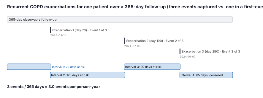
Patient 3041 has COPD and is followed for one full calendar year (January 1 through December 31, 2024) after starting a new inhaler. During that year the patient has three moderate-to-severe COPD exacerbations. We want to know the patient's annual exacerbation rate. A first-event-only analysis would record only the March flare-up and then stop watching — yielding a single event. The recurrent-events approach keeps watching and captures all three, giving an event rate of 3.0 exacerbations per person-year.

Dataset

Counting-process layout for patient 3041: one row per at-risk interval, each ending at the next exacerbation or the administrative end of follow-up. This is the format the Andersen-Gill model actually reads.

Steps

• Follow-up begins on day 0 (2024-01-01). The patient is at risk until the first exacerbation.

• The first exacerbation occurs on day 70 (2024-03-11). Row 1 ends here with event = 1.

• The patient re-enters the risk set immediately. The second exacerbation occurs 120 days later on day 190 (2024-07-09). Row 2 ends here with event = 1.

• The patient re-enters the risk set again. The third exacerbation occurs 90 days later on day 280 (2024-10-07). Row 3 ends here with event = 1.

• No further exacerbations occur. Follow-up closes at day 365 (2024-12-31) when the study ends. Row 4 ends here with event = 0 (administrative censoring).

• Total person-time = 365 days = 1.00 person-year. Total events = 3. Event rate = 3 divided by 1.00 = 3.0 exacerbations per person-year.

• A first-event-only Cox model would have stopped at row 1 and recorded only 1 event in 70 days, missing the two later flare-ups entirely.

Result

3 exacerbations in 365 days of follow-up = 3.0 events per person-year. A first-event analysis using only the day-70 event would see 1 event in 0.19 person-years and miss two-thirds of this patient's disease burden.

Timeline Spec

Title

Recurrent COPD exacerbations for one patient over a 365-day follow-up (three events captured vs. one in a first-event analysis)

Window

Start

2024-01-01

End

2024-12-31

Label

365-day observable follow-up

Events

• Label

  Exacerbation 1 (day 70)

  Start

  2024-03-11

  Length Days

  1

  Quantity

  Event 1 of 3

• Label

  Exacerbation 2 (day 190)

  Start

  2024-07-09

  Length Days

  1

  Quantity

  Event 2 of 3

• Label

  Exacerbation 3 (day 280)

  Start

  2024-10-07

  Length Days

  1

  Quantity

  Event 3 of 3

Spans

• Kind

  followup

  Start

  2024-01-01

  End

  2024-03-11

  Label

  Interval 1: 70 days at risk

• Kind

  followup

  Start

  2024-03-11

  End

  2024-07-09

  Label

  Interval 2: 120 days at risk

• Kind

  followup

  Start

  2024-07-09

  End

  2024-10-07

  Label

  Interval 3: 90 days at risk

• Kind

  followup

  Start

  2024-10-07

  End

  2024-12-31

  Label

  Interval 4: 85 days, censored

Result

Label

3 events / 365 days = 3.0 events per person-year

Value

3.0

Caption

Each diamond marks one COPD exacerbation. The four horizontal spans show the four at-risk intervals that make up the counting-process data rows. A first-event analysis would stop at the first diamond and ignore the two later events, understating this patient's burden by two-thirds.

Alt Text

A 365-day horizontal timeline for patient 3041 from January 1 to December 31, 2024. Three event markers appear at day 70 (March 11), day 190 (July 9), and day 280 (October 7), each labeled as an exacerbation. Four follow-up spans fill the gaps between events and the end of follow-up, illustrating the counting-process interval structure. A note indicates that a first-event-only analysis captures only the first marker and stops.

Runnable example

import numpy as np
import statsmodels.api as sm
import statsmodels.formula.api as smf

# Offset = log of observable person-time (in years here so the rate is events/person-year).
df["log_pt_years"] = np.log(df["pt_days"] / 365.25)

nb = smf.glm(
    formula="n_events ~ arm + age + cci",
    data=df,
    family=sm.families.NegativeBinomial(),      # absorbs within-person overdispersion
    offset=df["log_pt_years"],
    freq_weights=df["ps_weight"] if "ps_weight" in df else None,
).fit(cov_type="cluster", cov_kwds={"groups": df["person_id"]})

rr = np.exp(nb.params["arm"])
ci = np.exp(nb.conf_int().loc["arm"])
print(f"Rate ratio (arm) = {rr:.3f}  95% CI [{ci[0]:.3f}, {ci[1]:.3f}]")

from lifelines import CoxTimeVaryingFitter

ctv = CoxTimeVaryingFitter()
ctv.fit(
    long,
    id_col="person_id",
    start_col="tstart",
    stop_col="tstop",
    event_col="event",
    formula="arm + on_treatment + age + cci",
    robust=True,            # sandwich variance for within-person dependence (AG -> LWYY-style SE)
)
ctv.print_summary()         # exp(coef) on 'arm' is the recurrent-event rate/intensity ratio