Time-Updated Exposures and Cumulative Dose

In plain language

When researchers study how a drug affects the body over time, they need to track not just whether a patient ever took the drug, but exactly when the drug was active and how much had been taken up to each point. Time-updated exposure construction does this by dividing each patient's follow-up into small intervals and labeling each one with the exposure status at that moment — for example, whether a pill supply was currently on hand (current use) or how many total milligrams had accumulated up to that day (cumulative dose). This approach prevents a well-known counting error called immortal time bias, which occurs when a study incorrectly marks days before a patient even started the drug as if they were already exposed. Without it, a static ever/never label collapses the entire timeline into one flag and hides the most important information: the timing and amount of what was actually taken.

Real treatments are rarely a single fixed dose held over follow-up. Patients fill late, stockpile, titrate, switch route, pause for surgery, combine therapies, and discontinue for toxicity or cost. Time-updated exposure construction turns a stream of pharmacy fills, infusion administrations, or procedure claims into a person-time representation in which the exposure value assigned to each interval reflects what was actually being taken at that point in follow-up. This data step is not preprocessing to be rushed — it is the analysis. A correct estimand and a sophisticated model cannot rescue an exposure variable that mislabels person-time.

The common exposure scales, all defined as of a time `t` strictly before any outcome it could plausibly cause: current use (an active supply/administration episode covers `t`); recent use (exposure within a risk window, e.g. the prior 30 days, to capture carry-over pharmacology); cumulative duration (total exposed days before `t`); cumulative dose (sum of daily-dose × exposed days, or dispensed quantity, before `t`); dose intensity (cumulative dose per unit of exposed or protocol time); and weighted cumulative exposure (WCE), in which past doses contribute to current hazard through an estimated recency/latency weight function rather than a flat sum.

Core conceptual distinction

The decisive choice is what biologic quantity drives risk, and it dictates both the exposure variable and the estimand. A static `ever_exposed` flag answers "did this person ever take the drug" and, when used as a baseline covariate in a survival model, mislabels the unexposed lead-in as exposed (or forces follow-up to begin before the exposure decision), manufacturing immortal time. A time-varying current-use indicator answers "is risk elevated while on drug" (acute pharmacology); cumulative dose/duration answers "does risk accrue with total burden" (cumulative toxicity, e.g. anthracycline cardiomyopathy); WCE answers "how does the timing of past doses shape current risk" when a flat cumulative sum is biologically wrong (recent doses matter more, or a latency lag applies). These are not interchangeable: the estimand — a hazard ratio per active-use interval, per 1000 cumulative mg, or a WCE weight curve — must be pre-specified, and each maps to a different model (time-dependent Cox / pooled logistic on the long format, or, when the time-varying exposure is affected by prior outcomes/confounders, a marginal structural model fit by IPTW).

Pros, cons, and trade-offs

- vs static ever/never or baseline-only exposure: Time-updated exposure removes immortal time and the gross misclassification of pre-initiation and post-discontinuation person-time, and it lets the contrast match the pharmacology. Cost: it demands clean episode construction, lagging decisions, and far more programming; it is also vulnerable to treatment-by-indication feedback (dose is changed in response to evolving disease), which a naive time-dependent Cox cannot handle. Prefer for any safety/effectiveness question where exposure genuinely varies over follow-up. - vs PDC / MPR adherence summaries (pdc-proportion-of-days-covered): PDC collapses a fill history into one scalar over a fixed denominator — useful for an adherence predictor or descriptor, but it discards when exposure occurred and cannot represent time-varying risk. Time-updated exposure preserves the timeline. Cost: more complex, less standardized. Prefer PDC when adherence itself is the quantity of interest and timing is not; prefer time-updated when the hazard model needs interval-level exposure. - vs WCE specifically (within this family): A flat cumulative sum assumes every past mg counts equally forever; WCE relaxes that with a spline-weighted history and often fits short-latency or wash-in pharmacology far better. Cost: WCE needs dense exposure histories, is prone to overfitting sparse high-dose tails, and is harder to communicate to regulators than a pre-specified current-use or cumulative-dose contrast. Prefer WCE only when the flat-sum assumption is biologically indefensible and the data support estimating a weight curve. - vs marginal structural models (marginal-structural-models-g-methods): A standard time-dependent Cox on time-updated exposure is valid only when time-varying confounders are not themselves affected by prior exposure. When they are (e.g. labs that respond to the drug and also drive subsequent dosing), conditioning on them biases the effect and omitting them confounds it — the classic g-method trap. The exposure-history long format built here is the input to an MSM; the difference is the weighting/estimation layer, not the exposure construction. Escalate to an MSM/IPTW when that feedback exists.

When to use

Cumulative-toxicity questions (cumulative dose/duration: nephrotoxins, anthracyclines, opioids); acute on-treatment hazards (current/recent use: bleeding on anticoagulation, hypoglycemia on insulin); titrated or interrupted regimens where a baseline dose is meaningless by month three; as-treated arms of an active-comparator new-user or target-trial-emulation analysis that censor at switch/discontinuation; and any setting where setting time zero correctly still leaves exposure changing afterward.

When NOT to use — and when it is actively misleading or dangerous

Do not reach for time-varying exposure when the estimand is an initiation (intention-to-treat-like) contrast — there, exposure is fixed at time zero by design and adding post-baseline time-varying status re-introduces the very informative-censoring and mediator-adjustment problems the new-user design was built to avoid. It is actively dangerous to (1) feed cumulative dose into a model without lagging: using exposure measured up to and including the outcome day lets reverse causation and protopathic effects (the prodrome drives the prescription) masquerade as a dose-response, fabricating a spurious gradient; (2) update exposure using information that is a consequence of incipient disease, which conditions on a collider; (3) apply a standard time-dependent Cox when time-varying confounders are affected by prior treatment — this silently produces a biased estimate that looks rigorous. When dose is changed in response to the outcome process, only g-methods recover the causal effect.

Data-source operational depth

- Claims (FFS): Exposure episodes are built from `fill_date` + `days_supply` + daily dose derived from NDC strength and quantity. Real failure modes: (a) Medicare Advantage / capitated person-time lacks FFS fill claims, so any interval drawn from an MA-only member shows phantom "no current use" and a frozen cumulative dose — exclude MA-only person-time or restrict to Parts A/B/D (commercial: require an active pharmacy benefit), and treat the boundary as administrative censoring, not discontinuation. (b) 90-day mail-order and stockpiling inflate `days_supply` and apparent current use; decide a stockpiling/carry-over rule (cap accumulated supply) and a grace period explicitly. (c) Inpatient stays: most inpatient drugs are bundled and invisible to outpatient pharmacy, so an outpatient supply spanning a hospitalization may not reflect what was actually given — choose by design to bridge (assume continuation) or censor the stay, and report the choice. - EHR: "Current use" can come from the medication list (often stale, carried forward indefinitely), the order (intent, not receipt), the administration (MAR — true for inpatient infusions), or the e-prescribe feed (closest to a fill but missing whether it was picked up). These answer different questions; pick the source that matches the exposure definition (administrations for infusional oncology; linked fills for oral adherence) and never silently mix them. Visit- driven capture means a patient who leaves the system shows a spurious exposure gap — treat loss to follow-up as potentially informative. - Registry: Cycle-level dose and dose intensity are often captured more cleanly than in claims, but dose holds and reductions are frequently documented only in unstructured notes, so structured cycle data can overstate received dose; link to claims for complete outpatient fills/administrations and to a death index for censoring. - Linked claims–EHR–registry: The ideal substrate (registry dose + claims completeness + EHR labs to model feedback), but order/fill/administration date discrepancies must be reconciled before any interval boundary is set, and linkage selects the linkable subset.

Worked claims example

Question: dose-dependent risk of acute kidney injury (AKI) with an oral nephrotoxin, FFS claims. (1) Eligibility/time zero: first qualifying fill (`index_date`) after 365 days of continuous A/B/D enrollment and a drug-free washout; exclude members with any MA-only span in the lookback. (2) Build episodes: sort fills by `person_id`, `fill_date`; stitch with carry-over (start of fill `i` = `max(fill_date_i, covered_until_{i-1})`, `stop = start + days_supply`, daily dose from NDC strength × quantity / days_supply); cap stockpiled supply at 30 days; allow a 14-day grace before an episode is closed as discontinued. (3) Long format: split each person's follow-up at every episode boundary, every outcome/censoring date, and at the first day of each calendar month, emitting `(person_id, tstart, tstop, current_use, cum_days, cum_dose_mg)`. (4) Lag for latency/protopathic protection: compute `cum_dose_mg` and `current_use` as of `tstart` and lagged 30 days — exposure on the AKI day itself is excluded so a prodromal creatinine bump that triggers a refill cannot create false dose-response. (5) Censor: at disenrollment, death, end of data, and — for an as-treated contrast — at the end of the last episode + grace; bridge any inpatient stay by design and flag it. (6) Model: `coxph(Surv(tstart, tstop, aki) ~ cum_dose_100mg + current_use + baseline_covariates)` (or weighted pooled logistic), with the cumulative-dose coefficient reported per 100 mg; if creatinine both responds to the drug and drives subsequent dosing, escalate to an IPTW marginal structural model rather than adjusting for time-varying creatinine in the Cox model.

Worked example

Scenario

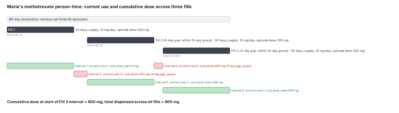
A researcher is studying whether long-term methotrexate use raises the risk of liver injury. She is following one patient, Maria (ID 2001), who started methotrexate on January 10, 2024. She has three pharmacy fills over about 100 days. Rather than label Maria as simply ever-exposed, the researcher builds a person-time table that records, for each interval of follow-up, whether Maria had an active supply on hand (current use = 1 or 0) and exactly how many total milligrams she had accumulated up to the start of that interval. This lets the survival model ask: does the liver-injury rate go up as cumulative dose grows?

Dataset

Maria's three pharmacy fills as they appear in a claims pharmacy table. Each row is one dispensed prescription.

Steps

• Fill 1 starts January 10 and covers 30 days, so it runs through February 8 (Jan 10 + 30 days). Maria has an active supply during this whole stretch. Episode dose = 30 days x 10 mg/day = 300 mg.

• Fill 2 arrives February 15. Her previous supply ended February 8, so there is a 6-day gap (Feb 9 through Feb 14). The 14-day grace period rule keeps this gap inside the same treatment episode rather than counting it as a restart, but during those 6 days current_use = 0 because no supply was on hand.

• Fill 2 restarts coverage on February 15 and runs through March 15 (30 days). Cumulative dose at the start of this interval is 300 mg (what was taken in Fill 1).

• Fill 3 arrives March 20. Supply from Fill 2 ended March 15, creating a 4-day gap (Mar 16 through Mar 19) where current_use = 0 again.

• Fill 3 restarts coverage March 20 through April 18. Cumulative dose at the start of this interval is 300 mg + 300 mg = 600 mg.

• By the end of Follow-up (April 18), Maria has completed all three fills. Total dose dispensed = 3 fills x 300 mg = 900 mg. A survival model can now ask whether the hazard of liver injury at any interval is higher when cumulative dose is 300 mg vs 600 mg vs 900 mg.

Result

At the start of the third fill interval (March 20), Maria's cumulative dose is 600 mg (Fill 1: 300 mg + Fill 2: 300 mg). Her current_use flag on March 20 is 1 (active supply). During the two gap intervals (Feb 9-14, Mar 16-19) current_use = 0, but cumulative dose continues to hold its running value of 300 mg and 600 mg respectively because dose already taken does not disappear.

Timeline Spec

Title

Maria's methotrexate person-time: current use and cumulative dose across three fills

Window

Start

2024-01-10

End

2024-04-18

Label

99-day observation window (all three fill episodes)

Events

• Label

  Fill 1

  Start

  2024-01-10

  Length Days

  30

  Quantity

  30 days_supply, 10 mg/day, episode dose 300 mg

• Label

  Fill 2 (6-day gap, within 14-day grace)

  Start

  2024-02-15

  Length Days

  30

  Quantity

  30 days_supply, 10 mg/day, episode dose 300 mg

• Label

  Fill 3 (4-day gap, within 14-day grace)

  Start

  2024-03-20

  Length Days

  30

  Quantity

  30 days_supply, 10 mg/day, episode dose 300 mg

Spans

• Kind

  exposed

  Start

  2024-01-10

  End

  2024-02-08

  Label

  Interval 1: current_use=1, cum_dose_start=0 mg

• Kind

  gap

  Start

  2024-02-09

  End

  2024-02-14

  Label

  Interval 2: current_use=0, cum_dose=300 mg (6-day gap, grace)

• Kind

  exposed

  Start

  2024-02-15

  End

  2024-03-15

  Label

  Interval 3: current_use=1, cum_dose_start=300 mg

• Kind

  gap

  Start

  2024-03-16

  End

  2024-03-19

  Label

  Interval 4: current_use=0, cum_dose=600 mg (4-day gap, grace)

• Kind

  exposed

  Start

  2024-03-20

  End

  2024-04-18

  Label

  Interval 5: current_use=1, cum_dose_start=600 mg

Result

Label

Cumulative dose at start of Fill 3 interval = 600 mg; total dispensed across all fills = 900 mg

Value

600

Caption

Each colored bar shows one fill; grey gaps show days without active supply (current_use=0). The cumulative-dose label on each interval shows how much Maria had taken before that interval began — the value a survival model would use as the exposure at that point in time.

Alt Text

Horizontal timeline for patient 2001 across 99 days showing three methotrexate fills as green bars, two grey gaps between fills, and a cumulative dose annotation on each interval (0 mg, 300 mg, 300 mg, 600 mg, 600 mg) demonstrating how the running total builds up across fills while current-use toggles on and off.

Runnable example

import pandas as pd

STOCKPILE_CAP_DAYS = 30   # max carry-over of unused supply
GRACE_DAYS = 14           # gap tolerated before an episode is closed as discontinued

def build_exposure_episodes(fills: pd.DataFrame) -> pd.DataFrame:
    fills = fills.sort_values(["person_id", "fill_date"])
    rows = []
    for pid, g in fills.groupby("person_id", sort=False):
        covered_until = None     # running end of stockpiled supply
        cum_dose = 0.0           # mg accrued so far for this person
        for r in g.itertuples():
            if covered_until is None or r.fill_date > covered_until + pd.Timedelta(days=GRACE_DAYS):
                start = r.fill_date                       # new episode
            else:
                carry = min((covered_until - r.fill_date).days, STOCKPILE_CAP_DAYS)
                start = r.fill_date + pd.Timedelta(days=max(carry, 0))   # cap stockpiling
            stop = start + pd.Timedelta(days=int(r.days_supply))
            episode_dose = int(r.days_supply) * float(r.daily_dose)
            rows.append({
                "person_id": pid, "tstart": start, "tstop": stop,
                "daily_dose": r.daily_dose, "current_use": 1,
                "cum_dose_start": cum_dose,                # cum dose BEFORE this episode (lag-ready)
                "cum_dose_end": cum_dose + episode_dose,
            })
            cum_dose += episode_dose
            covered_until = stop
    return pd.DataFrame(rows)

library(data.table)
library(survival)
STOCKPILE_CAP <- 30L; GRACE <- 14L

build_episodes <- function(fills) {
  setDT(fills); setorder(fills, person_id, fill_date)
  fills[, {
    covered_until <- as.Date(NA); cum <- 0; out <- list()
    for (i in seq_len(.N)) {
      fd <- fill_date[i]; ds <- days_supply[i]; dd <- daily_dose[i]
      if (is.na(covered_until) || fd > covered_until + GRACE) {
        start <- fd
      } else {
        carry <- min(as.integer(covered_until - fd), STOCKPILE_CAP)
        start <- fd + max(carry, 0L)
      }
      stop <- start + ds
      out[[i]] <- data.table(tstart = start, tstop = stop, daily_dose = dd,
                              current_use = 1L, cum_dose_start = cum)
      cum <- cum + ds * dd; covered_until <- stop
    }
    rbindlist(out)
  }, by = person_id]
}

epi <- build_episodes(fills)
# Restrict episodes to each person's follow-up and attach the event flag at the closing interval.
long <- epi[followup, on = .(person_id), nomatch = 0L][
  tstart < fu_end & tstop > fu_start]
long[, `:=`(tstart = pmax(tstart, fu_start), tstop = pmin(tstop, fu_end))]
long[, event := as.integer(!is.na(event_date) & event_date > tstart & event_date <= tstop)]
coxph(Surv(as.numeric(tstart), as.numeric(tstop), event) ~
        I(cum_dose_start / 100) + current_use, data = long)   # HR per 100 mg cumulative dose