Persistence Time to Discontinuation

In plain language

Persistence measures how long a patient keeps refilling a medication before stopping — specifically, the number of days from their first fill until the gap between when one supply ran out and the next fill arrived grew longer than an allowed limit (the permissible gap, commonly 30, 60, or 90 days). Unlike PDC, which asks how much medication a patient had on hand during a fixed window, persistence asks a simpler duration question: how many days did this person stay on therapy before quitting? One honest caveat: persistence built from pharmacy claims cannot see medications dispensed inside a hospital, free samples, or cash-paid fills, so those unobserved supply days may make a patient look like they stopped when they did not.

Persistence

is the duration phase of medication-taking behavior: how long a patient stays on a therapy after initiating it, ending when an allowable gap between the exhaustion of one fill's `days_supply` and the next fill exceeds a pre-specified threshold (the permissible gap, e.g., 30, 60, or 90 days). The day after the gap rule is breached becomes the discontinuation date; the interval from `index_date` to that date is the persistence time. Because every patient either discontinues, is censored (death, disenrollment, end of data), or remains persistent at study end, persistence is naturally a time-to-event outcome — not a ratio. The standardization literature (Cramer 2008, Vrijens ABC taxonomy 2012) is emphatic that this is a separate construct from adherence/implementation (PDC, MPR), which measures dose-taking intensity while the patient is still on therapy. A patient can be highly persistent (no qualifying gap for two years) yet poorly adherent (PDC of 0.55 from chronically late refills), and vice versa.

Core estimand distinction

. Persistence has two estimand layers that must be pre-specified, and conflating them is the most common error in the literature. (1) What event defines discontinuation — a permissible-gap breach on the index agent only (pure persistence), or a gap that is not bridged by a switch/add-on (treatment-episode persistence). (2) How competing events are handled — death and, in many designs, switching are competing risks that prevent the patient from ever being observed to discontinue the index drug. The naive Kaplan–Meier "persistence curve" treats death/disenrollment as non-informative censoring and therefore overstates the probability of remaining persistent when competing events are common (e.g., elderly oncology or heart-failure cohorts). The honest choices are the cause-specific hazard (rate of discontinuation among those still at risk and alive — answers an etiologic "why do people stop" question) versus the subdistribution hazard / cumulative incidence function (Fine–Gray — answers the prognostic "what fraction will be off drug by month 12" question, keeping those who died in the risk set). These are different numbers with different interpretations; report the CIF, not 1−KM, whenever competing risks are non-trivial.

Pros, cons, and trade-offs

. - vs pdc-proportion-of-days-covered (and mpr-medication-possession-ratio): Persistence captures time on therapy — the quantity that drives cumulative exposure, lines-of-therapy denominators, and the "on-treatment" windows for outcome assessment — whereas PDC/MPR capture intensity of supply over a fixed denominator and silently assume the patient is still on drug. Cost: persistence is acutely sensitive to the chosen gap length (Gardarsdottir 2010 shows episode counts and discontinuation rates swing materially from 30 to 90 days) and says nothing about adherence quality during the persistent period. Prefer persistence when the question is continuation/discontinuation, episode length, or defining on-treatment exposure; prefer PDC when the question is degree of adherence within a fixed window. - vs a binary "persistent at 12 months" proportion: The time-to-event formulation uses all the follow-up, respects differential censoring, and supports comparative hazard ratios; the binary endpoint discards timing and mishandles patients censored before the landmark. Prefer the survival formulation for almost all analytic work; reserve the binary version for simple descriptive reporting at a single, fully-observed landmark. - vs treatment-switch / switch-add-on-augmentation-rwe: Persistence logic supplies the gap machinery that switch and augmentation algorithms depend on, but the gap definition directly shapes switch classification — a short permissible gap inflates apparent discontinuations and restarts. Use persistence as the substrate, then layer switch rules on top with a consistent gap.

When to use

. Persistence (or non-persistence/time-to-discontinuation) as a primary or secondary endpoint in drug utilization, comparative effectiveness, or value-demonstration studies; constructing treatment episodes to define on-treatment exposure windows; CMS Star/PQA-style chronic-therapy continuation reporting; any setting with longitudinal dispensing dates and `days_supply`. Pair it with a survival model (Kaplan–Meier/cause-specific Cox for the etiologic contrast; Fine–Gray/CIF when death or switching competes).

When NOT to use — and when it is actively misleading or dangerous

. - No reliable dispensing/`days_supply` data. EHR prescription orders are not fills; persistence built on orders systematically overstates continuation because it cannot see primary non-adherence (an order never filled — see primary-non-adherence-initiation) or true discontinuation. Use linked pharmacy claims or treat order-based persistence as a different, weaker construct. - Competing risks ignored in a high-mortality cohort. Reporting 1−KM as "persistence" when death is frequent is actively misleading: it inflates apparent persistence and, if mortality differs by arm, biases the comparison. Switch to CIF/Fine–Gray or report cause-specific hazards with explicit handling of the competing event. - MA-only or capitated person-time. Persistence computed where pharmacy claims are not fully captured manufactures spurious gaps (a "discontinuation" that is really unobserved fills). Restrict to person-time with complete pharmacy benefit. - The real question is adherence intensity, not duration. A patient who fills sporadically but never opens a gap-length gap is "persistent"; if you care about whether they took enough drug, use PDC/MPR, not persistence. - Immortal-time in procedure/initiation framing. If follow-up or persistence start is set at a landmark before the index fill (e.g., diagnosis date), the pre-fill interval is immortal and biases the curve upward.

Data-source operational depth

. - Claims (FFS): The reference substrate — reliable `fill_date`, `days_supply`, and dispensed quantity. Require continuous medical + pharmacy enrollment from index through follow-up so absent fills are true gaps, not missingness. Real failure modes: 90-day mail-order and bulk fills distort gap timing (a single mail fill covers a stretch that looks like over-supply, and the next gap is mis-dated) — handle with carry-over/stockpiling rules capped at a maximum look-ahead; inpatient/SNF stays can bridge a gap if facility-administered drug is assumed (claims may not show a pharmacy fill during admission) — decide a priori whether hospitalization days suspend the gap clock; free samples and $0 copay cards are invisible. Censor at death, disenrollment, and end of data. - Claims (Medicare Advantage / capitated): MA-only person-time frequently lacks complete FFS pharmacy claims, so "no fill" is unobserved, not a true discontinuation — exclude MA-only spans or require Part D. In elderly claims, competing risks (death) differ by exposure, so a naive persistence curve compares non-comparable risk sets; CIF is mandatory, not optional. - EHR (orders only): Order-based "persistence" overstates continuation and cannot detect primary non-adherence; prefer linked dispensing. Visit-driven capture means a patient who leaves the system looks like a discontinuer — distinguish loss-to-follow-up from true stopping. - Linked claims–EHR / registry: Best of both — EHR/registry severity and mortality plus claims fill completeness — but linkage selects the linkable subset and introduces order/fill/service date discrepancies that must be reconciled before the gap clock starts. Registries strengthen the competing-event (death) ascertainment that the CIF needs.

Worked claims example

Question: 12-month persistence on a newly initiated oral antidiabetic in a commercial + Medicare FFS database, comparing two agents. (1) Cohort: adults with ≥2 type-2-diabetes diagnoses and 365 days of continuous medical + pharmacy enrollment before the first study fill (`index_date`); no fill of the index agent in that washout (new users). (2) Build the supply timeline: for each `person_id`, order pharmacy fills by `fill_date`; the covered interval of a fill runs from `fill_date` to `fill_date + days_supply`. Apply a carry-over rule — if a refill arrives before the prior supply is exhausted, push the leftover days forward (stockpiling), capped at, say, 30 surplus days to avoid implausible hoarding from 90-day mail fills. (3) Apply the gap rule: walk the timeline; the first time the next `fill_date` exceeds the running supply-end by ≥ the permissible gap (primary = 60 days; sensitivity = 30 and 90), discontinuation occurs on `supply_end + 1`. (4) Persistence time = `discontinuation_date − index_date`; patients with no qualifying gap are persistent and censored at the earliest of disenrollment, end of data, or day 365; death is a competing event, not plain censoring. (5) Estimate: Kaplan–Meier and cause-specific Cox for the etiologic discontinuation-rate contrast, and the cumulative incidence function (Fine–Gray) for the prognostic "fraction off drug by 12 months," because diabetes cohorts carry non-trivial mortality. (6) Report all three gap lengths; a conclusion that flips between 30- and 90-day gaps is a finding about the algorithm, not the drug.

Worked example

Scenario

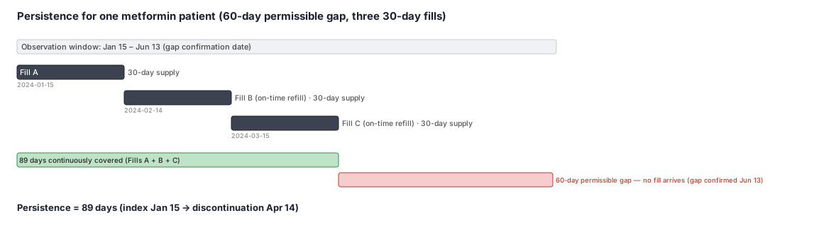
Maria starts metformin on January 15, 2024, for her type-2 diabetes. She refills on time twice. Then life gets busy — she never refills again. We are using a 60-day permissible gap: if no fill arrives within 60 days of the day her supply ran out, we call that discontinuation. How many days was Maria persistent on metformin?

Dataset

Raw rows an analyst would see in a claims pharmacy table for patient Maria (person_id 2001). Each row is one filled prescription.

Steps

• Fill A (Jan 15, 30-day supply) covers Jan 15 through Jan 44 — but January only has 31 days, so the last covered day is Feb 13. The supply runs out at the end of Feb 13; supply_end = Feb 14 (the first uncovered day).

• Fill B (Feb 14, 30-day supply) arrives exactly on the first uncovered day, so the gap is zero days. Supply now extends through Mar 14; supply_end = Mar 15.

• Fill C (Mar 15, 30-day supply) again arrives exactly on the first uncovered day, gap zero. Supply now extends through Apr 13; supply_end = Apr 14.

• No Fill D ever arrives. Starting Apr 14, the gap clock ticks. By Jun 12 (60 days later), still no fill — the permissible gap is breached.

• Discontinuation is backdated to Apr 14, the first day Maria had no supply (supply_end of Fill C). The gap was confirmed on Jun 13, but the event date is the earlier backdated date.

• Persistence = discontinuation date minus index date = Apr 14 minus Jan 15 = 89 days. Maria was persistent on metformin for 89 days.

Result

Label

Persistence = 89 days (Jan 15 to Apr 14, 60-day permissible gap)

Value

89

Pdc Contrast

PDC would ask a different question over a fixed window — say 180 days: how many of those 180 days did Maria have pills on hand? She had supply Jan 15 through Apr 13 = 89 covered days, so PDC = 89 / 180 = 0.49. Persistence says 'she lasted 89 days before stopping'; PDC says 'she had medication only 49 % of the time we were watching.' Both use the same fills — they just answer different questions. Use persistence when you care how long the patient stayed on therapy; use PDC when you care how fully they covered the treatment window.

Timeline Spec

Title

Persistence for one metformin patient (60-day permissible gap, three 30-day fills)

Window

Start

2024-01-15

End

2024-06-13

Label

Observation window: Jan 15 – Jun 13 (gap confirmation date)

Events

• Label

  Fill A

  Start

  2024-01-15

  Length Days

  30

  Quantity

  30-day supply

• Label

  Fill B (on-time refill)

  Start

  2024-02-14

  Length Days

  30

  Quantity

  30-day supply

• Label

  Fill C (on-time refill)

  Start

  2024-03-15

  Length Days

  30

  Quantity

  30-day supply

Spans

• Kind

  covered

  Start

  2024-01-15

  End

  2024-04-13

  Label

  89 days continuously covered (Fills A + B + C)

• Kind

  gap

  Start

  2024-04-14

  End

  2024-06-12

  Label

  60-day permissible gap — no fill arrives (gap confirmed Jun 13)

Result

Label

Persistence = 89 days (index Jan 15 → discontinuation Apr 14)

Value

89

Caption

Maria's three fills provide continuous coverage from Jan 15 through Apr 13 (89 days). After Fill C's supply runs out on Apr 13, no refill arrives within the 60-day permissible window. The gap is confirmed on Jun 13, but discontinuation is backdated to Apr 14 — the first day she had no supply. Persistence = Apr 14 minus Jan 15 = 89 days. PDC over this same 89-day span would be 89/89 = 1.0 while she was on therapy, but PDC over a fixed 180-day window would be 89/180 = 0.49.

Alt Text

A horizontal timeline showing three consecutive 30-day fill bars (Fill A Jan 15, Fill B Feb 14, Fill C Mar 15) shaded as covered days, followed by a 60-day gap bar starting Apr 14 with no fill arriving. A marker labeled 'Discontinuation Apr 14' sits at the start of the gap bar. The total persistent period is annotated as 89 days.

Runnable example

import pandas as pd
import numpy as np
from lifelines import AalenJohansenFitter

PERMISSIBLE_GAP = 60      # days beyond supply exhaustion that defines discontinuation (sensitivity: 30, 90)
MAX_CARRYOVER = 30        # cap on surplus days carried forward (guards against 90-day mail-fill over-supply)
HORIZON = 365             # administrative landmark

def time_to_discontinuation(fills: pd.DataFrame, index: pd.DataFrame, outcome: pd.DataFrame) -> pd.DataFrame:
    f = fills.merge(index[["person_id", "index_date"]], on="person_id")
    f = f[f["fill_date"] >= f["index_date"]].sort_values(["person_id", "fill_date"])

    rows = []
    for pid, g in f.groupby("person_id"):
        supply_end = None                       # running covered-through date (with carry-over)
        disc_date = None
        for fill_date, dsup in zip(g["fill_date"], g["days_supply"]):
            if supply_end is None:
                supply_end = fill_date + pd.Timedelta(days=int(dsup))
                continue
            gap = (fill_date - supply_end).days
            if gap >= PERMISSIBLE_GAP:           # gap rule breached -> discontinued the day after supply ran out
                disc_date = supply_end + pd.Timedelta(days=1)
                break
            carry = max(min((supply_end - fill_date).days, MAX_CARRYOVER), 0)  # leftover supply, capped
            supply_end = fill_date + pd.Timedelta(days=int(dsup) + carry)
        rows.append({"person_id": pid, "last_supply_end": supply_end, "disc_date": disc_date})

    epi = pd.DataFrame(rows).merge(index, on="person_id").merge(outcome, on="person_id")

    # Competing-risks status: 1 = discontinuation, 2 = death before discontinuation, 0 = censored.
    admin = epi["index_date"] + pd.Timedelta(days=HORIZON)
    cens = epi[["disenroll_date", "end_date"]].min(axis=1).fillna(admin).clip(upper=admin)
    disc = epi["disc_date"]
    death = epi["death_date"]

    status = np.zeros(len(epi), dtype=int)
    event_date = cens.copy()
    # earliest of discontinuation / death / censor wins
    d_disc = disc.fillna(pd.Timestamp.max)
    d_death = death.fillna(pd.Timestamp.max)
    disc_first = (d_disc <= cens) & (d_disc <= d_death)
    death_first = (d_death <= cens) & (d_death < d_disc)
    status = np.where(disc_first, 1, np.where(death_first, 2, 0))
    event_date = np.where(disc_first, d_disc, np.where(death_first, d_death, cens))
    epi["status"] = status
    epi["persistence_days"] = (pd.to_datetime(event_date) - epi["index_date"]).dt.days.clip(lower=0, upper=HORIZON)
    return epi[["person_id", "arm", "persistence_days", "status"]]

def cif_discontinuation(epi: pd.DataFrame) -> AalenJohansenFitter:
    # Cumulative incidence of discontinuation (event 1) with death (event 2) as competing risk.
    ajf = AalenJohansenFitter()
    ajf.fit(epi["persistence_days"], epi["status"], event_of_interest=1)
    return ajf

library(data.table)
library(survival)
library(cmprsk)

PERMISSIBLE_GAP <- 60L; MAX_CARRYOVER <- 30L; HORIZON <- 365L

persistence_episodes <- function(fills, index, outcome) {
  setDT(fills); setDT(index); setDT(outcome)
  f <- merge(fills, index[, .(person_id, index_date)], by = "person_id")
  f <- f[fill_date >= index_date][order(person_id, fill_date)]

  disc <- f[, {
    supply_end <- NA; disc_date <- as.Date(NA)
    for (i in seq_len(.N)) {
      if (is.na(supply_end)) { supply_end <- fill_date[i] + days_supply[i]; next }
      gap <- as.integer(fill_date[i] - supply_end)
      if (gap >= PERMISSIBLE_GAP) { disc_date <- supply_end + 1L; break }
      carry <- max(min(as.integer(supply_end - fill_date[i]), MAX_CARRYOVER), 0L)
      supply_end <- fill_date[i] + days_supply[i] + carry
    }
    .(disc_date = disc_date)
  }, by = person_id]

  epi <- Reduce(function(a, b) merge(a, b, by = "person_id"), list(disc, index, outcome))
  admin <- epi$index_date + HORIZON
  cens  <- pmin(epi$disenroll_date, epi$end_date, admin, na.rm = TRUE)

  d_disc  <- fifelse(is.na(epi$disc_date),  as.Date("9999-12-31"), epi$disc_date)
  d_death <- fifelse(is.na(epi$death_date), as.Date("9999-12-31"), epi$death_date)
  disc_first  <- d_disc  <= cens & d_disc  <= d_death
  death_first <- d_death <= cens & d_death <  d_disc
  epi[, status := fifelse(disc_first, 1L, fifelse(death_first, 2L, 0L))]
  evt <- fifelse(disc_first, d_disc, fifelse(death_first, d_death, cens))
  epi[, persistence_days := pmin(pmax(as.integer(evt - index_date), 0L), HORIZON)]
  epi[, .(person_id, arm, persistence_days, status)]
}

# Cause-specific Cox (etiologic) and Fine-Gray subdistribution (prognostic CIF) for the index-drug contrast.
fit_persistence <- function(epi) {
  cs <- coxph(Surv(persistence_days, status == 1L) ~ arm, data = epi)   # cause-specific hazard of discontinuation
  fg <- crr(epi$persistence_days, epi$status, cov1 = model.matrix(~ arm, epi)[, -1, drop = FALSE], failcode = 1, cencode = 0)
  list(cause_specific = cs, fine_gray = fg)
}