Continuous Enrollment and Observable Time
The requirement that a person be under continuous data capture (enrolled in a health plan, or within an EHR/registry observation window) across each baseline and follow-up interval, so that the absence of a record can be interpreted as the absence of the event rather than as unobserved care.
On this page
A claims database records events — doctor visits, hospital stays, filled prescriptions — only while a person is actively enrolled in a health plan. When enrollment lapses, the database goes silent: it cannot tell you whether the person had no events or simply had events that went unrecorded. Continuous enrollment is the rule that a patient must have an unbroken coverage record across every analysis window, so that 'no record of an event' can honestly be read as 'no event.' The catch is that requiring perfect, unbroken coverage shrinks your study group and can favor healthier, more stably employed people.
Continuous enrollment / observable time
is the data-availability requirement that underlies almost every other operational decision in claims, EHR, and registry research. A subject contributes valid observable person-time only during intervals in which the data source is actually capturing that person's care. In claims, observability means active enrollment with the relevant benefit (medical and pharmacy, for the lines of business that flow claims); in EHR it means an open observation period at a site that records the encounters of interest; in registries it means an active follow-up status with the data elements being abstracted. Outside those intervals, the data are silent, and silence is not the same as "no event."
Core conceptual distinction — observability vs. occurrence
The entire validity of count-based and time-to-event RWE rests on the assumption that, within observable time, absence of a claim/record equals absence of the event. Continuous enrollment is what makes that assumption defensible. It governs three separate things that beginners conflate:
- the baseline lookback — you can only assert "no prior diagnosis/treatment" if the person was observable throughout the lookback (this is what a washout requires);
- follow-up person-time — the denominator for rates and the time-at-risk for survival models must be restricted to observable intervals, or you systematically miss events that occurred off-plan; and
- outcome ascertainment — an outcome that happens during an unobserved gap is misclassified as a non-event. The concept is therefore the data-observability precondition for the washout (`washout-clean-lookback-period-rwe`), the person-time denominator (`person-time-denominator-construction-rwe`), and time-zero alignment (`time-zero-index-date-alignment-rwe`); those concepts assume continuous enrollment has already been established.
Pros, cons, and trade-offs
- vs. no enrollment requirement (use everyone with any claim): Requiring continuous enrollment removes the most common source of differential outcome misclassification in claims (events that fall in coverage gaps are coded as non-events) and makes lookback-based exclusions honest. Cost: it shrinks the cohort, skews it toward the continuously insured (typically healthier, more stably employed, or older Medicare-eligible), and can erode generalizability. Prefer a continuous-enrollment requirement for any rate, incidence, or survival endpoint; relax it only for cross-sectional prevalence on a fixed date where prior observability is irrelevant.
- vs. strict zero-gap enrollment: A small, pre-specified gap tolerance (e.g., allow one gap of <=45 days, bridged by assuming continuity) recovers people who churn briefly between plans or have administrative coverage lapses, increasing power and representativeness. Cost: a tolerated gap is a window of true non-observability — events in it are still missed, biasing rates downward — so the tolerance must be small relative to the outcome's detectability window and reported. Prefer a modest, transparent gap rule over strict zero-gap when churn is common, but never tolerate gaps longer than the induction/latency window of the outcome.
- vs. as-treated or registry-driven observability: Continuous plan enrollment is the right observability frame for claims; for EHR/registry the analogous frame is the observation period (`omop-observation-period-rwe`), which is inferred from encounter density rather than an explicit enrollment field and is therefore softer and more error-prone. Prefer enrollment fields when available; reconstruct observation periods only when no enrollment table exists, and validate them against known-capture events (e.g., annual wellness visits).
When NOT to use / when it is actively misleading
- Immortal-time creation. Defining the cohort so that survival from index to a later qualifying event (e.g., requiring a fixed post-index enrollment minimum, or requiring a second fill to confirm exposure) guarantees subjects were event-free and observable over that interval. If that interval is counted as exposed/at-risk, it manufactures immortal time bias (`immortal-time-bias-handling`) — the classic trap in procedure and adherence studies. Start follow-up at time zero and let enrollment censor, never select, follow-up.
- Medicare Advantage (MA) person-time treated as observable. MA encounter data are notoriously incomplete and, in many research extracts, MA enrollees do not generate the fee-for-service (FFS) claims that downstream code assumes. Counting MA-only spans as observable makes "no event" largely an artifact of missing claims — events and prior treatments simply do not appear. Restrict to Parts A+B (and D for drug exposure) FFS, and exclude MA-only person-time, or the entire rate is biased toward the null.
- Differential observability by exposure. If one arm is enrolled/captured more completely than the other (e.g., a drug requiring specialty-pharmacy enrollment, or a comparator concentrated in a churning Medicaid population), continuous enrollment differs by arm and the resulting differential ascertainment mimics a treatment effect. Diagnose by comparing enrollment duration and gap distributions across arms.
- Coverage gap that swallows the outcome. For an acute, quickly-fatal, or out-of-network-treated outcome (e.g., out-of-area MI, hospice care), enrollment may technically continue while the capturing benefit does not, or the event is paid outside the observed plan. Continuous enrollment is necessary but not sufficient; pair it with a mortality source hierarchy (`mortality-source-hierarchy-rwe`) and out-of-network capture checks.
Data-source operational depth
- Claims (commercial / Medicare FFS / Medicaid): Observable time = enrollment spans with the right benefit. Require both medical and pharmacy enrollment whenever exposure is a drug, because medical-only enrollees never generate pharmacy claims and would falsely pass a drug washout. Reconcile the raw monthly eligibility table into continuous spans, apply the gap rule, and intersect every analysis window with these spans. Failure modes: MA-only person-time lacking FFS claims (above); plan switching that fragments enrollment within the same person; mid-month enrollment booleans that overstate coverage; capitated/bundled arrangements where services are paid without itemized claims; and adjudication lag at the end of data that mimics a coverage gap (truncate follow-up before the run-out window). In Medicaid, frequent churn makes a strict zero-gap rule discard a large, non-random share of the cohort.
- EHR: There is no enrollment field; observability is inferred from encounter activity (the OMOP observation period or a "first/last note" window). A patient who seeks care elsewhere is differentially lost without any signal, so "no record of diagnosis X" can mean off-system care, not absence. Define observation windows explicitly, prefer sites/systems with high capture, link to claims to confirm continuity, and treat loss to follow-up as potentially informative (`attrition-and-loss-to-follow-up-rwe`).
- Registry: Observability = active follow-up status with the elements being abstracted; completeness varies by visit schedule and site. Link to claims for interval health-care use between registry visits and to a death index to firm up censoring. Registry "no event" between scheduled visits is interval-censored, not point-observed.
- Linked claims–EHR–vital records: The strongest substrate — enrollment from claims gives true observability windows, EHR adds severity, vital records firm up mortality — but linkage restricts to the linkable subset (selection) and creates date discrepancies (enrollment span vs. encounter date vs. service date) that must be reconciled before any window is intersected.
Worked claims example
Question: 12-month incidence of hospitalized acute pancreatitis among new initiators of a GLP-1 receptor agonist in a commercial + Medicare FFS database.
- Build observable spans: collapse the monthly eligibility table into continuous enrollment spans requiring both medical and pharmacy benefit; exclude any MA-only months so that absence of a claim is genuine.
- Apply a gap rule: treat the person as continuously enrolled if any enrollment gap is <=45 days, bridging it as covered; a single longer gap truncates the span.
- Baseline observability / washout: require 365 days of continuous observable time before the first GLP-1 fill (`fill_date`) so the new-user (no prior GLP-1) and exclusion (no prior pancreatitis `dx` in any position) criteria are verifiable, not assumed.
- Time zero = that first qualifying `fill_date`.
- Follow-up person-time: accrue at-risk time from time zero only while the observable span is open; right-censor at the earliest of first hospitalized pancreatitis (>=1 inpatient claim with the qualifying `dx` in the primary position), disenrollment / end of the observable span, death (from the mortality hierarchy), or 365 days — and stop follow-up before the claims run-out window to avoid mistaking adjudication lag for a coverage gap.
- First-event coding: count only the first qualifying event per person; deduplicate same-episode inpatient claims.
- Diagnostics: report the attrition funnel (continuous-enrollment requirement is typically the largest single exclusion), the enrollment-gap distribution, person-time by arm, and a sensitivity analysis varying the gap tolerance (0, 30, 45 days) and the lookback length to show the rate is not an artifact of the observability rule.
Decision diagram
flowchart TD
  Elig[Monthly eligibility table<br/>medical / pharmacy / MA flags] --> Drop[Drop MA-only months<br/>require medical AND pharmacy]
  Drop --> Span[Collapse into continuous spans<br/>bridge gaps <= tolerance]
  Span --> Look[Full lookback observable?<br/>span_start <= index - 365d]
  Look -->|yes| T0[Time zero = first qualifying fill]
  Look -->|no| Excl[Exclude: prior period unobservable<br/>washout cannot be verified]
  T0 --> Fup[Accrue at-risk time only while span open<br/>censor at span end / death / run-out]
  Fup --> Asc[Outcome ascertainment within observable time<br/>no record = no event]
gantt
  title Observable time vs. silent time for one subject (claims)
  dateFormat YYYY-MM-DD
  axisFormat %b %Y
  section Enrollment
  Continuous medical + pharmacy (observable) :done, obs1, 2023-01-01, 2023-09-30
  Coverage gap (silent - events MISSED)      :crit, gap, 2023-10-01, 45d
  Re-enrolled (observable)                   :done, obs2, 2023-11-15, 2024-12-31
  section Design windows
  365d lookback / washout (must be observable) :active, lb, 2023-01-01, 2023-12-31
  Time zero = first qualifying fill            :milestone, t0, 2024-01-01, 0d
  Follow-up at-risk (observable only)          :active, fu, 2024-01-01, 270d
Worked example
Scenario
Patient 1001 is enrolled in a commercial health plan for most of 2023, but their coverage lapses for 45 days in the fall. We want to count hospital admissions over a January 1 – December 31, 2023 observation window. We need to know which days are truly observable, how many person-days the patient contributes, and what happens to an event that falls inside the gap.
Dataset
Raw monthly enrollment rows for patient 1001 — each row represents one calendar month of active coverage.
| person_id | elig_month | medical | pharmacy |
|---|---|---|---|
| 1001 | 2023-01-01 | True | True |
| 1001 | 2023-02-01 | True | True |
| 1001 | 2023-03-01 | True | True |
| 1001 | 2023-04-01 | True | True |
| 1001 | 2023-05-01 | True | True |
| 1001 | 2023-06-01 | True | True |
| 1001 | 2023-07-01 | True | True |
| 1001 | 2023-08-01 | True | True |
| 1001 | 2023-09-01 | True | True |
| 1001 | 2023-11-01 | True | True |
| 1001 | 2023-12-01 | True | True |
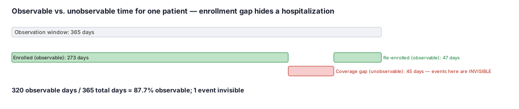
Steps
Result
- Label
Observable days / Total window days
- Value
320 / 365 = 87.7% of the year was observable; the 45-day gap is genuine unobservable time, and the October 20 hospitalization is invisible to the study.
Trade-offs
Runnable example
Build continuous observable-time spans from a monthly eligibility table, then derive each subject's baseline lookback, time zero, and at-risk follow-up restricted to observable time. Required inputs (already cleaned, de-duplicated): elig : monthly enrollment -> person_id, elig_month (period 'M'), medical (bool),...
import pandas as pd
import numpy as np

LOOKBACK_DAYS = 365   # continuous observable time required before index
GAP_TOLERANCE = 45    # bridge enrollment gaps <= this many days
RUNOUT_DAYS   = 90    # claims adjudication run-out; do not follow patients into it

def build_observable_spans(elig: pd.DataFrame) -> pd.DataFrame:
    """Collapse monthly eligibility into continuous spans with BOTH medical+pharmacy
    benefit, excluding MA-only months, and bridging gaps <= GAP_TOLERANCE days."""
    e = elig[elig["medical"] & elig["pharmacy"] & (~elig["ma_only"])].copy()
    e["start"] = e["elig_month"].dt.to_timestamp()                       # first day of month
    e["end"]   = (e["elig_month"] + 1).dt.to_timestamp() - pd.Timedelta(days=1)  # last day
    e = e.sort_values(["person_id", "start"])

    # A new span begins when the gap from the prior covered month exceeds the tolerance.
    prev_end = e.groupby("person_id")["end"].shift()
    gap = (e["start"] - prev_end).dt.days
    e["new_span"] = (gap.isna()) | (gap > GAP_TOLERANCE + 1)
    e["span_id"]  = e.groupby("person_id")["new_span"].cumsum()
    spans = (e.groupby(["person_id", "span_id"])
               .agg(span_start=("start", "min"), span_end=("end", "max"))
               .reset_index())
    return spans

def build_cohort(elig: pd.DataFrame, rx: pd.DataFrame, study_class: str,
                 data_end: pd.Timestamp) -> pd.DataFrame:
    spans = build_observable_spans(elig)

    # Candidate index = first fill of the study drug class.
    idx = (rx[rx["drug_class"] == study_class]
             .sort_values(["person_id", "fill_date"])
             .groupby("person_id", as_index=False).first()
             .rename(columns={"fill_date": "index_date"}))[["person_id", "index_date"]]

    # Attach the observable span that CONTAINS the index date.
    cand = idx.merge(spans, on="person_id")
    cand = cand[(cand["span_start"] <= cand["index_date"]) &
                (cand["span_end"]   >= cand["index_date"])]

    # Require LOOKBACK_DAYS of continuous observable time before index within that span.
    cand["baseline_start"] = cand["index_date"] - pd.Timedelta(days=LOOKBACK_DAYS)
    cand = cand[cand["span_start"] <= cand["baseline_start"]].copy()

    # Follow-up is censored at the end of the observable span, the data run-out, never later.
    admin_end = data_end - pd.Timedelta(days=RUNOUT_DAYS)
    cand["fup_end"] = cand[["span_end"]].assign(admin=admin_end).min(axis=1)
    return cand[["person_id", "index_date", "baseline_start", "fup_end"]]
Same logic with data.table. Inputs mirror the Python version: elig : person_id, elig_month (Date, first of month), medical (logical), pharmacy (logical), ma_only (logical) rx : person_id, fill_date (Date), drug_class (character), days_supply (integer) Returns one row per eligible new initiator: index_date,...
library(data.table)
LOOKBACK_DAYS <- 365L
GAP_TOLERANCE <- 45L
RUNOUT_DAYS   <- 90L

build_observable_spans <- function(elig) {
  e <- as.data.table(elig)[medical & pharmacy & !ma_only]
  e[, start := elig_month]                                  # first day of month
  e[, end   := seq(elig_month, by = "month", length.out = 2)[2] - 1, by = .I]  # last day of month
  setorder(e, person_id, start)
  # New span when the gap from the prior covered month exceeds the tolerance.
  e[, prev_end := shift(end), by = person_id]
  e[, gap := as.integer(start - prev_end)]
  e[, new_span := is.na(gap) | gap > GAP_TOLERANCE + 1L]
  e[, span_id := cumsum(new_span), by = person_id]
  e[, .(span_start = min(start), span_end = max(end)), by = .(person_id, span_id)]
}

build_cohort <- function(elig, rx, study_class, data_end) {
  spans <- build_observable_spans(elig)
  rx <- as.data.table(rx)
  setorder(rx, person_id, fill_date)
  idx <- rx[drug_class == study_class, .(index_date = fill_date[1L]), by = person_id]

  cand <- merge(idx, spans, by = "person_id", allow.cartesian = TRUE)
  cand <- cand[span_start <= index_date & span_end >= index_date]            # span containing index
  cand[, baseline_start := index_date - LOOKBACK_DAYS]
  cand <- cand[span_start <= baseline_start]                                 # full lookback observable
  admin_end <- data_end - RUNOUT_DAYS
  cand[, fup_end := pmin(span_end, admin_end)]                              # censor at span end / run-out
  cand[, .(person_id, index_date, baseline_start, fup_end)]
}
Build continuous observable-time spans and the new-initiator cohort in SAS. Required inputs (post data-management): work.elig : person_id, elig_month (date, first of month), medical (0/1), pharmacy (0/1), ma_only (0/1) work.rx : person_id, fill_date (date), drug_class (char), days_supply (num) Macro vars set the...
%let lookback = 365;
%let gaptol   = 45;
%let runout   = 90;
%let dataend  = '31DEC2024'd;

/* Keep only months with BOTH benefits and exclude MA-only person-time; build month spans. */
data elig_keep;
  set work.elig;
  if medical=1 and pharmacy=1 and ma_only=0;
  mstart = elig_month;
  mend   = intnx('month', elig_month, 1) - 1;   /* last day of the eligibility month */
  format mstart mend date9.;
run;
proc sort data=elig_keep; by person_id mstart; run;

/* Collapse months into continuous spans, bridging gaps <= &gaptol days. */
data spans;
  set elig_keep; by person_id mstart;
  retain span_start span_end;
  prev_end = lag(mend);
  if first.person_id then do; span_start=mstart; span_end=mend; end;
  else if (mstart - prev_end) > (&gaptol + 1) then do;
    output;                       /* close previous span */
    span_start=mstart; span_end=mend;
  end;
  else span_end = max(span_end, mend);
  if last.person_id then output;  /* close final span */
  keep person_id span_start span_end;
  format span_start span_end date9.;
run;

/* Candidate index = first fill of the study drug class. */
proc sql;
  create table idx as
  select person_id, min(fill_date) as index_date format=date9.
  from work.rx where drug_class = "STUDY"
  group by person_id;
quit;

/* Index must fall inside an observable span with the full lookback covered; censor at span end / run-out. */
proc sql;
  create table cohort as
  select i.person_id,
         i.index_date,
         i.index_date - &lookback                  as baseline_start format=date9.,
         min(s.span_end, &dataend - &runout)       as fup_end        format=date9.
  from idx i
  inner join spans s
    on i.person_id = s.person_id
   and s.span_start <= i.index_date
   and s.span_end   >= i.index_date
   and s.span_start <= i.index_date - &lookback;   /* full lookback observable within the span */
quit;
Citations
- [1]Schneeweiss S, Avorn J. A review of uses of health care utilization databases for epidemiologic research on therapeutics. Journal of Clinical Epidemiology. 2005;58(4):323-337.
- [2]Hall GC, Sauer B, Bourke A, Brown JS, Reynolds MW, LoCasale RJ. Guidelines for good database selection and use in pharmacoepidemiology research. Pharmacoepidemiology and Drug Safety. 2012;21(1):1-10.
- [3]Suissa S. Immortal time bias in pharmacoepidemiology. American Journal of Epidemiology. 2008;167(4):492-499.