Person-Time Denominator Construction

In plain language

When a study follows people over time to count new disease events, the denominator of the rate is not the number of people — it is the total amount of time all those people were actually being watched and were at risk of having the event. Each participant contributes days from the moment they enter the study until they either have the event, leave the study, or the data run out; those individual stretches of time are then added together to form the denominator. This total accumulated follow-up time (called the time-at-risk) is expressed in person-days or person-years, and dividing the event count by it gives the incidence rate. The approach handles real-world messiness naturally, because people who are followed for different lengths of time each contribute only as much time as they were actually observed.

Person-time denominator construction

is the operational machinery that turns a cohort of subjects into the denominator of a rate: it decides, for every individual, when their clock starts, when it stops, and which intervals of calendar, age, and time-since-exposure that follow-up gets credited to. The numerator of an incidence rate is a count of events; the denominator is the sum of at-risk time over everyone who could have had the event. Get the time-at-risk wrong and the rate is wrong, regardless of how cleanly the outcome was ascertained. In RWE this is rarely a one-line `time = exit - entry` calculation — it is enrollment spans intersected with exposure episodes intersected with the at-risk window, then Lexis-split so that a piecewise-constant rate can be estimated on the right scale.

Core conceptual distinction

. Three anatomical decisions define the denominator and are separable. (1) Origin (time zero): the index/treatment-initiation date for an incident-user analysis, or diagnosis/enrollment for a natural-history cohort. Person-time accrued before the exposure could possibly act must not be credited to the exposure — doing so is the mechanism of immortal time bias, where survivors are guaranteed event-free until they qualify and that "immortal" span is misallocated to the treated denominator, deflating its rate. (2) Exit and the censoring hierarchy: follow-up ends at the first of the outcome event, a competing event (e.g., death when the outcome is a non-fatal hospitalization), administrative end-of-data, loss of observability (disenrollment), and — for an as-treated estimand — treatment discontinuation or switch. Which exits stop the clock versus count as the event is an estimand decision, not a programming detail. (3) Time-scale splitting (the Lexis diagram): the hazard is almost never constant on a single scale, so a person's interval is cut at age-band boundaries, calendar-year boundaries, and time-since-initiation boundaries, producing multiple (tstart, tstop, event) rows per person. Each row contributes its person-time to one cell; rates are then estimated per cell or modeled with these counting-process records (`Surv(tstart, tstop, event)`), which is also exactly the input a time-dependent Cox model consumes. The estimand distinction matters: an intention-to-treat (initiation) denominator credits all post-time-zero observable time to the assigned arm regardless of later switching; an as-treated denominator credits only on-treatment time (days_supply stitched with grace periods, censored at discontinuation/switch) and usually requires inverse-probability-of-censoring weighting because discontinuation is informative.

Pros, cons, and trade-offs

. - vs a naive `exit - entry` single-interval denominator: Explicit interval construction (enrollment ∩ exposure ∩ at-risk) prevents crediting unobservable or post-exit time and prevents immortal time. Cost: substantially more programming and diagnostics. Prefer interval construction for any rate that informs a regulatory or HTA decision. - vs unsplit person-time with a single average rate: Lexis splitting lets the rate vary by age, calendar time, and time-since-exposure and is mandatory for direct/indirect standardization and for time-dependent hazard models. Cost: a larger, multi-row analytic table and care that no person-time is double-counted across cells. Prefer splitting whenever the rate plausibly changes on a scale you care about (it almost always does with age and follow-up duration). - vs cumulative-incidence (risk) denominators: A rate denominator (person-time) handles staggered entry, variable follow-up, and censoring naturally and is the right tool when follow-up length differs across subjects; a risk denominator (persons at baseline) answers "what fraction by time t" and needs competing-risk handling (cumulative incidence function). Prefer person-time rates for sparse events with heterogeneous follow-up; prefer risk/CIF when an absolute probability over a fixed horizon is the decision-relevant quantity and competing events are common.

When to use

. Any incidence-rate, mortality-rate, or event-rate estimate from longitudinal RWE with variable follow-up; as the denominator for direct or indirect standardization (SMR/SIR); as the counting-process input to time-dependent Cox or Poisson/negative-binomial rate models; whenever subjects enter at different calendar times, are observed for different durations, or move between exposure states during follow-up.

When NOT to use — and when it is actively misleading or dangerous

. - When the decision quantity is an absolute probability over a fixed horizon with substantial competing risk. A rate per 1,000 person-years can be multiplied into a misleading "risk" by ignoring that death removes people from the at-risk set; report the cumulative incidence function instead. In elderly claims cohorts where the competing risk of death differs by exposure arm, naive rate comparisons are actively misleading about absolute burden. - When immortal time is being silently credited. If time zero is set at diagnosis but exposure is defined by a later prescription, the gap is immortal and must either be excluded, treated as unexposed, or handled with a time-dependent exposure. Crediting it to the exposed denominator manufactures a spurious protective effect — the classic Suissa failure mode in procedure and prescription studies. - When the denominator includes unobservable time. Counting calendar time during which the data source cannot see events (a disenrolled gap, an MA-only span with no fee-for-service claims) inflates the denominator and deflates the rate. This is a denominator error masquerading as a low event rate. - When prevalent subjects enter with unaccounted left truncation. Registry cohorts that enroll prevalent cases start the clock after the origin; treating them as if observed from origin biases rate estimates (late-entry / delayed-entry must be modeled).

Data-source operational depth

. - Claims (FFS): Person-time is the intersection of continuous medical/pharmacy enrollment spans with the at-risk window. Require continuous enrollment so that absence of a claim is true absence, not unobservability. Failure modes: (a) Medicare Advantage (MA)-only spans carry no fee-for-service claims — events are invisible there, so that calendar time must be removed from the denominator (censor at MA entry), not assumed event-free; drop the person-time, not the person. (b) Plan-switch and coverage gaps create unobservable intervals — split the at-risk interval at the gap and exclude it. (c) Adjudication/run-out lag means the most recent months of claims are incomplete; truncate the study end before the lag horizon or person-time near the end is under-eventful. (d) 90-day mail-order and stockpiling distort as-treated on-treatment windows and grace-period stitching. - EHR: Capture is visit-driven, so absence of an encounter is not evidence of no event — a patient who silently leaves the system contributes apparent event-free person-time that is really unobserved. Define an observability window (e.g., recent encounter within N months) and treat loss to follow-up as potentially informative censoring; link to pharmacy/claims to confirm exposure episodes. - Registry: Strong for adjudicated outcomes and severity but often enrolls prevalent subjects, inducing left truncation; the at-risk clock must start at the true origin with delayed entry, and registry completeness/linkage eligibility define which person-time is observable. - Linked claims–EHR–vital records: The ideal substrate, but order, fill, and service dates disagree; reconcile them before assigning time zero and interval boundaries, and recognize that only the linkable subset contributes person-time (linkage selection).

Worked claims example

Question: incidence rate of acute kidney injury (AKI) among new SGLT2 inhibitor initiators aged ≥65 in fee-for-service Medicare. (1) Origin / time zero: first SGLT2i fill (NDC + `fill_date`), with ≥365 days of continuous Parts A/B/D FFS enrollment before it (washout confirms incident use and observability). (2) At-risk start: time zero. (3) At-risk exit = first of: validated AKI dx (the event), death (a competing event — stops the clock, not counted as AKI), disenrollment or MA entry (censor — unobservable thereafter), end of data minus the 3-month adjudication lag, and — for the as-treated denominator — last `days_supply` end + a 30-day grace period or switch to another antidiabetic. (4) Compute person-time: for each person, `person_days = at_risk_exit - time_zero` over observable, on-treatment spans, split at each calendar-year and age-band boundary. (5) Arithmetic: suppose across the cohort there are 240 first AKI events and the summed observable on-treatment time is 511,000 person-days. Person-years = 511,000 / 365.25 = 1,398.8. Incidence rate = 240 / 1,398.8 × 1,000 = 171.6 per 1,000 person-years (95% CI from the Poisson/exact interval). Note how excluding MA-only and disenrolled spans lowers the denominator and raises the rate versus a naive `enroll_end - time_zero` denominator that would have silently counted unobservable time.

Interpreting the output

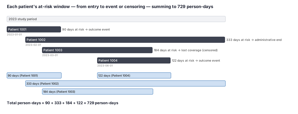
Denominator construction for a 4-patient cohort yields 729 observable at-risk person-days (90 + 333 + 184 + 122), with 2 events; the resulting incidence rate denominator is 729 person-days (approximately 2.0 person-years).

Formal interpretation. Each patient contributes person-time only during intervals satisfying three conditions: (1) active enrollment in a plan type with observable claims — Medicare FFS or commercial; MA-only periods are excluded because utilization is unobservable; (2) the patient has not yet experienced the outcome; and (3) the observation falls within the at-risk window defined by time zero and censoring rules. The 729-person-day total is the denominator for the incidence rate, not the 4-patient head count. Patients contribute different amounts of time because of staggered entry, variable follow-up, and administrative censoring. Lexis-splitting at calendar-year and age-band boundaries enables age- and calendar-stratified rates from the same denominator dataset.

Practical interpretation. Misspecifying the denominator — for example, using enrollment end rather than the MA-exclusion-aware at-risk exit date — silently inflates observed time and underestimates the true event rate. The correct 729-person-day denominator is the foundation of any subsequent incidence rate, rate ratio, or standardized rate calculation. Report total person-time, mean and range of individual follow-up, and the number and reason for each type of censoring so that reviewers can audit the at-risk construction independently.

Worked example

Scenario

A claims database study is tracking new users of a blood-pressure drug to measure how often they develop a kidney problem (the outcome event) in 2023. Four patients start the drug at different times during the year. The analyst needs to figure out how much time each patient was actually being observed and at risk, then sum those amounts to build the denominator of the incidence rate.

Dataset

One row per patient showing their entry date, the date their follow-up ended, why it ended, and the number of days they were at risk (exit date minus entry date).

Steps

• Patient 1001 entered 2023-01-01 and had the kidney event on 2023-04-01 — the clock stops on the event date, giving 90 days at risk (Jan: 31 + Feb: 28 + Mar: 31 = 90).

• Patient 1002 entered 2023-02-01 and was still event-free when the study data ended on 2023-12-31 — this is an administrative end, not an event, so their 333 days count fully in the denominator.

• Patient 1003 entered 2023-03-01 but lost insurance coverage on 2023-09-01, meaning the database can no longer see their events — the clock is stopped at that date (censored) after 184 days (Mar: 31 + Apr: 30 + May: 31 + Jun: 30 + Jul: 31 + Aug: 31 = 184).

• Patient 1004 entered 2023-06-01 and had the kidney event on 2023-10-01 — the clock stops on the event date, giving 122 days at risk (Jun: 30 + Jul: 31 + Aug: 31 + Sep: 30 = 122).

• Sum all four contributions: 90 + 333 + 184 + 122 = 729 person-days total time-at-risk — this is the denominator.

• Two outcome events occurred (patients 1001 and 1004), so the crude incidence rate = 2 events / 729 person-days = 0.00274 events per person-day, or equivalently 2 / (729 / 365.25) = 2 / 1.995 person-years ≈ 1.003 events per person-year (roughly 1,003 per 1,000 person-years in this tiny four-patient illustration).

Result

Total time-at-risk = 90 + 333 + 184 + 122 = 729 person-days. Two events occurred. Incidence rate = 2 events / 729 person-days.

Timeline Spec

Title

Each patient's at-risk window — from entry to event or censoring — summing to 729 person-days

Window

Start

2023-01-01

End

2023-12-31

Label

2023 study period

Events

• Label

  Patient 1001

  Start

  2023-01-01

  Length Days

  90

  Quantity

  90 days at risk → outcome event

• Label

  Patient 1002

  Start

  2023-02-01

  Length Days

  333

  Quantity

  333 days at risk → administrative end

• Label

  Patient 1003

  Start

  2023-03-01

  Length Days

  184

  Quantity

  184 days at risk → lost coverage (censored)

• Label

  Patient 1004

  Start

  2023-06-01

  Length Days

  122

  Quantity

  122 days at risk → outcome event

Spans

• Kind

  followup

  Start

  2023-01-01

  End

  2023-04-01

  Label

  90 days (Patient 1001)

• Kind

  followup

  Start

  2023-02-01

  End

  2023-12-31

  Label

  333 days (Patient 1002)

• Kind

  followup

  Start

  2023-03-01

  End

  2023-09-01

  Label

  184 days (Patient 1003)

• Kind

  followup

  Start

  2023-06-01

  End

  2023-10-01

  Label

  122 days (Patient 1004)

Result

Label

Total person-days = 90 + 333 + 184 + 122 = 729 person-days

Value

729

Caption

Each horizontal bar shows one patient's at-risk window from their entry date to whichever exit came first — an outcome event (patients 1001 and 1004), administrative study end (patient 1002), or loss of insurance coverage (patient 1003). The lengths of the four bars add up to exactly 729 person-days, which is the denominator of the incidence rate.

Alt Text

Gantt-style timeline showing four horizontal bars for patients 1001 through 1004, each starting at a different date in 2023 and ending at different points; bar lengths of 90, 333, 184, and 122 days are labeled, and a summary note shows they sum to 729 person-days.

Runnable example

import pandas as pd
import numpy as np
from scipy.stats import chi2  # exact Poisson CI

def observable_at_risk(cohort: pd.DataFrame, enroll: pd.DataFrame) -> pd.DataFrame:
    """Intersect [time_zero, exit_date) with FFS-observable (non-MA) enrollment spans."""
    e = enroll[~enroll["ma_only"]].merge(
        cohort[["person_id", "time_zero", "exit_date", "event"]], on="person_id")
    # Clip each enrollment span to the at-risk window.
    e["seg_start"] = e[["enroll_start", "time_zero"]].max(axis=1)
    e["seg_end"]   = e[["enroll_end", "exit_date"]].min(axis=1)
    e = e[e["seg_end"] > e["seg_start"]].copy()
    # The event only counts on the segment that actually contains exit_date.
    e["event"] = np.where((e["event"] == 1) & (e["seg_end"] == e["exit_date"]), 1, 0)
    return e[["person_id", "seg_start", "seg_end", "event"]]

def split_calendar_year(seg: pd.DataFrame) -> pd.DataFrame:
    """Lexis split each observable segment at Jan-1 boundaries -> one row per (person, year)."""
    rows = []
    for r in seg.itertuples(index=False):
        start, end = r.seg_start, r.seg_end
        for yr in range(start.year, end.year + 1):
            lo = max(start, pd.Timestamp(yr, 1, 1))
            hi = min(end,   pd.Timestamp(yr + 1, 1, 1))
            if hi <= lo:
                continue
            ev = int(r.event == 1 and hi == end)  # event flag only on terminal sub-row
            rows.append((r.person_id, yr, (hi - lo).days, ev))
    return pd.DataFrame(rows, columns=["person_id", "cal_year", "person_days", "event"])

def incidence_rate(split: pd.DataFrame, per: int = 1000) -> pd.DataFrame:
    g = split.groupby("cal_year").agg(events=("event", "sum"),
                                      person_days=("person_days", "sum")).reset_index()
    g["person_years"] = g["person_days"] / 365.25
    g["rate"] = g["events"] / g["person_years"] * per
    # Exact (Garwood) Poisson 95% CI on the count, rescaled to PY.
    lo = chi2.ppf(0.025, 2 * g["events"]) / 2
    hi = chi2.ppf(0.975, 2 * (g["events"] + 1)) / 2
    g["lcl"] = lo / g["person_years"] * per
    g["ucl"] = hi / g["person_years"] * per
    return g

seg   = observable_at_risk(cohort, enroll)
split = split_calendar_year(seg)
print(incidence_rate(split))

library(survival)

## Follow-up time in years from time zero; counting-process form (tstart, tstop, event).
cohort$fu_years <- as.numeric(cohort$texit - cohort$t0) / 365.25
cohort$tstart   <- 0

## Lexis split on the follow-up time scale at 1-year cut points (also splittable on age via a second call).
cuts  <- seq(0, ceiling(max(cohort$fu_years)), by = 1)
split <- survSplit(Surv(fu_years, event) ~ ., data = cohort,
                   cut = cuts, start = "tstart", end = "tstop", episode = "fu_band")
split$pyears <- split$tstop - split$tstart  # person-years contributed by this sub-interval

## Crude rate per 1,000 PY with an exact Poisson interval.
pt <- sum(split$pyears); d <- sum(split$event)
rate <- d / pt * 1000
ci   <- poisson.test(d, T = pt)$conf.int * 1000
cat(sprintf("IR = %.1f per 1,000 PY (95%% CI %.1f-%.1f)\n", rate, ci[1], ci[2]))

## Rate model: Poisson with log person-time offset (rate ratio by arm and follow-up band).
fit_rate <- glm(event ~ arm + factor(fu_band) + offset(log(pyears)),
                family = poisson, data = split[split$pyears > 0, ])

## Same denominator, hazard model: time-dependent Cox on the counting-process rows.
fit_cox  <- coxph(Surv(tstart, tstop, event) ~ arm, data = split)