As-Treated Risk Window Construction

In plain language

An as-treated risk window marks exactly the days a patient had a drug on hand and counts only those days when attributing side effects or outcomes to the drug. You project each prescription fill forward by the number of days it is supposed to last, stitch consecutive fills together when a new fill arrives before the previous one runs out (or within a short grace period), and close the window when the patient goes too long without refilling. Any event that happens inside the window is charged to the drug; any event outside the window — after the patient has stopped — is not, because the drug was no longer acting. The method cannot see cash-paid fills or free samples, so gaps in the data may look like the patient stopped when they actually kept taking the drug.

As-treated (on-treatment) risk window construction

is the operational step that turns a stream of exposure records into time at risk: the spans of follow-up during which a patient is counted as actively exposed. It answers three coupled questions — when does exposed person-time start (almost always at the index fill/order, i.e. time zero), when is a patient still on treatment (supply-interval stitching, grace periods, carryover of oversupply), and when does exposed person-time end (run-out, discontinuation, switch, or the structural censoring events of disenrollment, death, and end of data). It is the engine behind an as-treated / per-protocol estimand and is distinct from an intention-to-treat (ITT) / first-line analysis that attributes all post-initiation follow-up to the initial drug regardless of later behavior.

Core conceptual / estimand distinction

The risk-window rule is the estimand made concrete. Under ITT you count outcomes for the whole observation window from time zero; the rule is trivial (one window per person) but the contrast is the effect of starting a strategy and dilutes with discontinuation and switching. Under as-treated you censor (or split) person-time when the patient leaves the protocol, so the contrast approaches the effect of staying on the drug — but only validly if you weight for the informative censoring that discontinuation/switching induce (inverse-probability-of-censoring weighting, IPCW). A naive as-treated analysis with no IPCW silently conditions on staying treated, which is a post-baseline variable on the causal pathway, and is biased whenever prognosis predicts who stays. The window rule also fixes the lag/induction structure — whether the first N days after initiation are "at risk" (acute outcomes) or excluded (latency for chronic outcomes) — and whether an outcome during a grace-period extension or a post-discontinuation "legacy" window still counts (carryover, depletion of the pharmacologic effect).

Pros, cons, and trade-offs

- vs intention-to-treat / first-line attribution: As-treated targets the biologically interpretable on-treatment effect, recovers dose-response and acute toxicities that ITT washes out, and matches the labeling question "what happens while a patient takes this." Cost: it requires careful episode logic and IPCW; done naively it reintroduces selection bias and is less defensible than a clean ITT. Prefer ITT for the policy/adherence question and as the primary in a target-trial emulation; prefer as-treated as the per-protocol companion or when the mechanism is acute and on-treatment timing dominates. - vs a single fixed risk window (e.g. "90 days after the index fill" for everyone): A fixed window is simple, immune to gap-rule arbitrariness, and standard for acute, single-dose, or vaccine-style exposures. Cost: it misclassifies person-time for chronic refilled therapy — patients who refilled for two years get 90 days, patients who stopped at day 10 get 90 days. Prefer fixed windows for acute/one-shot exposures and as a sensitivity analysis; prefer stitched as-treated windows for chronic, refillable drugs. - vs current-vs-former-vs-never time-updated exposure (the fuller g-method machinery): Time-updated exposure with a marginal structural model handles time-varying confounding affected by prior treatment that as-treated censoring cannot. Cost: far heavier specification and data demands. Prefer the as-treated window when discontinuation is not strongly confounded by evolving prognosis; escalate to time-updated/MSM when it is. - Grace period is the central nuisance parameter. Too short and you create artifactual gaps, fragment one true episode into many, and manufacture immortal/"unexposed" time between fills; too long and you carry exposure status far past the last pill, misattributing late events to a drug no longer present. The grace period must be pre-specified and varied in sensitivity analysis — it is the single choice most likely to move a hazard ratio.

When to use

Comparative safety where the hazard tracks active pharmacology (e.g., bleeding on an anticoagulant, hypoglycemia on a sulfonylurea), dose-response questions, per-protocol arms of a target-trial emulation, and any ITT analysis whose effect is suspected to be diluted by heavy discontinuation. Use it whenever "off-drug" person-time should not count as exposed.

When NOT to use — and when it is actively misleading or dangerous

- When discontinuation/switching is strongly driven by evolving prognosis and you do not weight for it. Sick patients stop drugs (or are stopped by clinicians); naive as-treated censoring then makes the remaining on-treatment time look healthier than it is — a textbook healthy-adherer / informative-censoring bias. If you cannot estimate censoring weights, an ITT primary is safer and more honest. - For chronic-effect or carcinogenic outcomes with long latency. Counting only current on-treatment time, with no induction lag and no legacy window, biases toward the null because the relevant etiologic exposure occurred years earlier. Use exposure-lag/induction windows or cumulative-dose metrics instead. - In procedure or hospitalization studies where the window is anchored to a future event. Defining "exposed" time using post-index information (e.g., counting the days until a procedure that only treated patients receive) creates immortal time — guaranteed event-free survival assigned to the exposed arm. The window must be built only from information available at its start. - In data that cannot observe the off-drug state. If supply, stop dates, or enrollment are not reliably captured, a "discontinuation" is indistinguishable from data loss and the window boundaries are noise.

Data-source operational depth

- Claims (FFS): Exposure spans come from pharmacy claims (`ndc`, `fill_date`, `days_supply`). The standard construction: sort fills per `person_id`, project each fill forward by `days_supply`, and if the next `fill_date` falls within the supply end plus the grace period, stitch the two into one continuous episode; otherwise close the episode at `supply_end + grace` (or at the last supply end). Carryover/stockpiling: when an early refill overlaps unused supply, shift the new supply start to the prior supply end so on-hand days accumulate (capped to avoid implausible hoarding). Failure modes and workarounds: (1) Medicare Advantage / capitated person-time lacks FFS pharmacy claims — an MA enrollee's "gap" is missingness, not discontinuation; restrict to Parts A/B/D (or commercial pharmacy benefit) and exclude MA-only spans. (2) 90-day mail-order and sample fills distort `days_supply`, lengthening or hiding episodes. (3) Inpatient days suppress outpatient pharmacy claims even though the drug is administered; bridge known inpatient stays so they are not scored as gaps. (4) Last fill near death leaves leftover supply that should be censored at death, not carried forward. - EHR: Exposure is the order or administration, not a paid claim; an active prescription with no fill is not on-treatment. e-Prescribing and medication-administration records help, but external-care leakage (fills at pharmacies outside the system) makes apparent discontinuation unreliable; link to dispensing where possible and treat loss to follow-up as potentially informative. Encounter-driven capture means the absence of a stop note is not evidence of continued use. - Registry: Often records treatment lines or start/stop at adjudicated visits but rarely day-level supply; derive coarse windows from visit-anchored start/stop and link to claims for granular refill stitching. - Linked claims–EHR–vital records: The ideal substrate — EHR start dates + claims fill completeness + a death index for the right-censoring boundary — but order/fill/service-date discrepancies must be reconciled before the window is built, or episodes will start and end on the wrong dates.

Competing risks within the window

In elderly claims populations, death is a frequent and differentially distributed competing event: an exposure that delays death lengthens on-treatment person-time and inflates the observed rate of any non-fatal outcome. Decide explicitly whether death censors the window (cause-specific) or is a competing event (subdistribution); a cause-specific window with differential mortality by arm can mislead.

Worked claims example

Question: rate of major GI bleeding while on low-dose aspirin in a Medicare FFS + commercial cohort. (1) Eligibility / time zero: first aspirin fill (`index_date`) after ≥365 days continuous A/B/D (or commercial medical+pharmacy) enrollment with no aspirin fill in the lookback (incident user). (2) Window start: day after `index_date` (or `index_date` itself, pre-specified); apply a 1-day induction so a bleed coded on the index day is not attributed to a drug not yet taken. (3) Stitching: for each subsequent fill, `supply_end = fill_date + days_supply`; if the next `fill_date <= supply_end + 30` (30-day grace), continue the episode and, if `fill_date < supply_end`, carry the unused days forward (cap total on-hand at 90 days). (4) Window end (censor exposed time at the earliest of): last `supply_end + 30`-day grace run-out (discontinuation), switch to a different antiplatelet (NDC change), disenrollment, death, or end of data. (5) Bridging: any inpatient stay overlapping a stitched episode is treated as on-treatment (drug administered in hospital), not a gap. (6) Outcome: first inpatient claim with a primary GI-bleed `dx` during open on-treatment person-time; person-time and events outside open windows are excluded (or contribute to an "off-treatment" comparison group). (7) Sensitivity: rerun with grace = 0/15/60 days, induction = 0/7 days, a 30-day post-discontinuation legacy window, and IPCW for informative discontinuation; report how the rate and any comparative HR move with each.

Worked example

Scenario

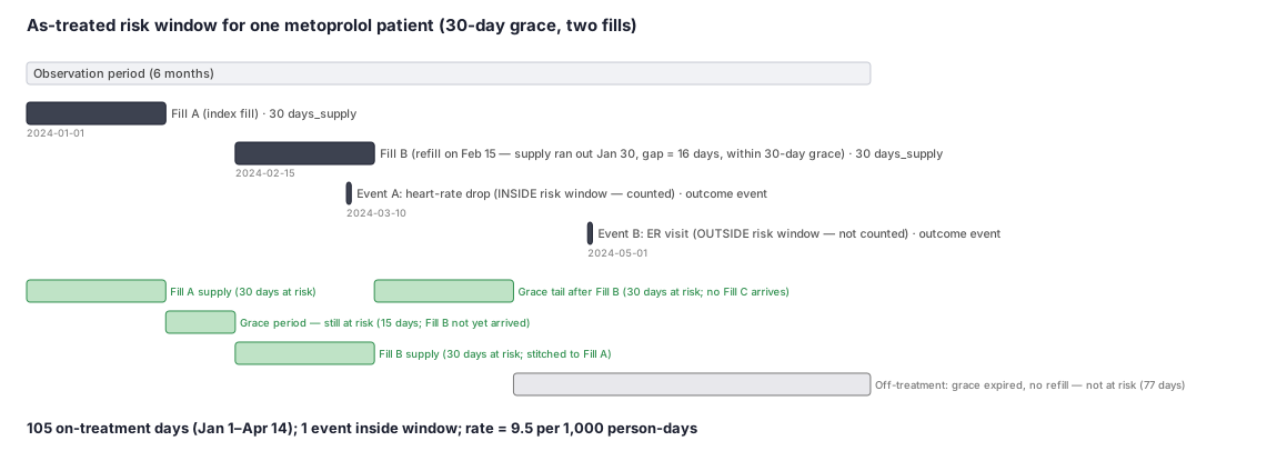
Patient 2001 is newly started on metoprolol (a blood pressure pill) on January 1, 2024. She fills it twice before stopping. We want to know which days count as 'at risk' — meaning the drug was plausibly in her system — so we can correctly attribute a heart-rate event to the drug only if it happened while she was actually taking it. We use a 30-day grace period: if her next fill arrives within 30 days of her supply running out, the two fills are joined into one unbroken risk window.

Dataset

Pharmacy claims rows for patient 2001 — exactly the columns an analyst sees in a real table.

Steps

• Fill A (Jan 1, 30-day supply) covers Jan 1 through Jan 30 — those 30 days are inside the risk window.

• After Jan 30 the supply is gone, but the 30-day grace period keeps the window open through Feb 29 while we wait to see if she refills.

• Fill B arrives on Feb 15, which is before the grace expires (Feb 29) — so the two fills are stitched into one continuous episode; no gap is recorded.

• Fill B's 30-day supply runs from Feb 15 through Mar 15; the 30-day grace tail then extends the window through Apr 14.

• No Fill C arrives by Apr 14, so the episode closes on Apr 14 — all days from Apr 15 onward are off-treatment.

• Event A (heart-rate drop, Mar 10) falls inside the risk window (Jan 1–Apr 14) and is counted as an on-treatment event.

• Event B (a separate ER visit, May 1) falls outside the closed window and is NOT counted as an on-treatment event — the drug was no longer acting.

• Total on-treatment days: Jan 1–Apr 14 = 31 (Jan) + 29 (Feb, leap year) + 31 (Mar) + 14 (Apr 1-14) = 105 days.

• Incidence rate = 1 on-treatment event ÷ 105 on-treatment days × 1,000 = 9.5 events per 1,000 person-days.

Result

105 on-treatment days; 1 event inside the window; incidence rate = 9.5 events per 1,000 person-days. Event B (May 1) does not contribute because the risk window closed on Apr 14.

Timeline Spec

Title

As-treated risk window for one metoprolol patient (30-day grace, two fills)

Window

Start

2024-01-01

End

2024-06-30

Label

Observation period (6 months)

Events

• Label

  Fill A (index fill)

  Start

  2024-01-01

  Length Days

  30

  Quantity

  30 days_supply

• Label

  Fill B (refill on Feb 15 — supply ran out Jan 30, gap = 16 days, within 30-day grace)

  Start

  2024-02-15

  Length Days

  30

  Quantity

  30 days_supply

• Label

  Event A: heart-rate drop (INSIDE risk window — counted)

  Start

  2024-03-10

  Length Days

  1

  Quantity

  outcome event

• Label

  Event B: ER visit (OUTSIDE risk window — not counted)

  Start

  2024-05-01

  Length Days

  1

  Quantity

  outcome event

Spans

• Kind

  exposed

  Start

  2024-01-01

  End

  2024-01-30

  Label

  Fill A supply (30 days at risk)

• Kind

  exposed

  Start

  2024-01-31

  End

  2024-02-14

  Label

  Grace period — still at risk (15 days; Fill B not yet arrived)

• Kind

  exposed

  Start

  2024-02-15

  End

  2024-03-15

  Label

  Fill B supply (30 days at risk; stitched to Fill A)

• Kind

  exposed

  Start

  2024-03-16

  End

  2024-04-14

  Label

  Grace tail after Fill B (30 days at risk; no Fill C arrives)

• Kind

  unexposed

  Start

  2024-04-15

  End

  2024-06-30

  Label

  Off-treatment: grace expired, no refill — not at risk (77 days)

Result

Label

105 on-treatment days (Jan 1–Apr 14); 1 event inside window; rate = 9.5 per 1,000 person-days

Value

105

Caption

Two fills are stitched into one 105-day risk window because Fill B arrives before the 30-day grace expires. Event A (Mar 10) lands inside and is attributed to metoprolol. Event B (May 1) lands in the off-treatment gap and is excluded from the on-treatment rate. If the grace period were shorter — say 10 days — Fill B would arrive too late to stitch and the single window would close Jan 30, cutting 75 days of legitimate at-risk time and possibly missing Event A entirely.

Alt Text

Horizontal timeline from January 1 to June 30, 2024. A blue exposed bar covers January 1 through April 14, subdivided into Fill A supply (Jan 1–Jan 30), a grace-period segment (Jan 31–Feb 14), Fill B supply (Feb 15–Mar 15), and a grace tail (Mar 16–Apr 14). A red event marker on March 10 sits inside the blue bar labeled 'Event A — counted.' A grey unexposed bar runs April 15 through June 30. A second red event marker on May 1 sits inside the grey bar labeled 'Event B — not counted.'

Runnable example

import pandas as pd
import numpy as np

GRACE_DAYS = 30      # permissible gap between fills before an episode is closed
CARRYOVER_CAP = 90   # max stockpiled on-hand days (guards against implausible hoarding)

def build_at_windows(rx: pd.DataFrame, censor: pd.DataFrame) -> pd.DataFrame:
    rx = rx.sort_values(["person_id", "fill_date"]).copy()
    episodes = []

    for pid, g in rx.groupby("person_id"):
        # Earliest structural censoring date for this person (NaT-safe min).
        c = censor.loc[censor["person_id"] == pid, ["disenroll_date", "death_date", "data_end"]]
        hard_stop = c.min(axis=1).min() if len(c) else pd.NaT

        ep_start = None
        on_hand_end = None     # running supply-end including carried-over days
        ep_drug = None

        for _, f in g.iterrows():
            start = f["fill_date"]
            supply_end = start + pd.Timedelta(days=int(f["days_supply"]))

            if ep_start is None:
                ep_start, on_hand_end, ep_drug = start, supply_end, f["drug_class"]
                continue

            # Switch closes the current episode at run-out + grace.
            switched = f["drug_class"] != ep_drug
            within_grace = start <= on_hand_end + pd.Timedelta(days=GRACE_DAYS)

            if within_grace and not switched:
                # Carry forward unused supply (stockpiling), capped.
                base = max(on_hand_end, start)
                on_hand_end = min(base + pd.Timedelta(days=int(f["days_supply"])),
                                  start + pd.Timedelta(days=CARRYOVER_CAP))
            else:
                episodes.append((pid, ep_drug, ep_start,
                                 on_hand_end + pd.Timedelta(days=GRACE_DAYS)))
                ep_start, on_hand_end, ep_drug = start, supply_end, f["drug_class"]

        if ep_start is not None:
            episodes.append((pid, ep_drug, ep_start,
                             on_hand_end + pd.Timedelta(days=GRACE_DAYS)))

    out = pd.DataFrame(episodes,
                       columns=["person_id", "drug_class", "episode_start", "episode_end"])
    # Right-censor every episode end at the structural stop (disenroll / death / data end).
    out = out.merge(
        censor.assign(hard_stop=censor[["disenroll_date", "death_date", "data_end"]].min(axis=1))
              [["person_id", "hard_stop"]],
        on="person_id", how="left")
    out["episode_end"] = out[["episode_end", "hard_stop"]].min(axis=1)
    out = out[out["episode_end"] > out["episode_start"]]   # drop empty windows
    return out.drop(columns="hard_stop").reset_index(drop=True)

library(data.table)
GRACE_DAYS    <- 30L
CARRYOVER_CAP <- 90L

build_at_windows <- function(rx, censor) {
  setDT(rx); setDT(censor)
  setorder(rx, person_id, fill_date)

  one_person <- function(g) {
    ep_start <- on_hand_end <- ep_drug <- NULL
    eps <- list()
    for (i in seq_len(nrow(g))) {
      start <- g$fill_date[i]
      supply_end <- start + g$days_supply[i]
      if (is.null(ep_start)) {
        ep_start <- start; on_hand_end <- supply_end; ep_drug <- g$drug_class[i]; next
      }
      switched     <- g$drug_class[i] != ep_drug
      within_grace <- start <= on_hand_end + GRACE_DAYS
      if (within_grace && !switched) {
        base <- max(on_hand_end, start)                      # carry unused supply forward
        on_hand_end <- min(base + g$days_supply[i], start + CARRYOVER_CAP)
      } else {
        eps[[length(eps) + 1L]] <- list(ep_drug, ep_start, on_hand_end + GRACE_DAYS)
        ep_start <- start; on_hand_end <- supply_end; ep_drug <- g$drug_class[i]
      }
    }
    eps[[length(eps) + 1L]] <- list(ep_drug, ep_start, on_hand_end + GRACE_DAYS)
    data.table(drug_class   = vapply(eps, `[[`, "", 1L),
               episode_start = as.Date(vapply(eps, function(e) as.numeric(e[[2L]]), 0), origin = "1970-01-01"),
               episode_end   = as.Date(vapply(eps, function(e) as.numeric(e[[3L]]), 0), origin = "1970-01-01"))
  }

  out <- rx[, one_person(.SD), by = person_id]
  hs  <- censor[, .(hard_stop = pmin(disenroll_date, death_date, data_end, na.rm = TRUE)),
                by = person_id]
  out <- merge(out, hs, by = "person_id", all.x = TRUE)
  out[!is.na(hard_stop), episode_end := pmin(episode_end, hard_stop)]
  out[episode_end > episode_start, .(person_id, drug_class, episode_start, episode_end)]
}