OMOP Time-at-Risk and Cohort Exit

In plain language

When researchers study whether a drug causes a health event, they need to define exactly which days each patient was being watched for that event -- this span is called the time-at-risk window. The window opens at the patient's starting point (usually the day they first took the drug, sometimes one day later to exclude events already present on that day) and closes at whichever comes first: a fixed number of follow-up days, the day the patient lost insurance coverage, or the day the outcome actually occurred. Getting these boundaries right lets the study count real new events rather than old ones, and avoids crediting a drug with event-free time that happened before anyone was even taking it.

In the OHDSI/OMOP framework a cohort is a set of persons who satisfy entry criteria for a span of time, and the analytic estimate is generated only over the time-at-risk (TAR) window attached to each cohort entry. TAR is defined by two offsets relative to anchor dates: a start rule (e.g., `cohort_start_date + start_date_offset`, often offset 0 = exposure initiation, or +1 day to exclude prevalent outcomes coded on the index day) and an end rule (`cohort_end_date`, `observation_period_end_date`, `drug_era_end_date + grace`, a fixed offset such as +365 days, or the first outcome). Cohort exit is the operationalization of that end rule plus all competing reasons follow-up stops — death, disenrollment, the end of the database, switching, or the outcome itself. TAR start, cohort exit, and the censoring source together fix the denominator (person-time) and which numerator (outcome) events are eligible to be counted. Get them wrong and you do not get a noisier estimate of the right thing — you get a precise estimate of the wrong thing.

Core conceptual distinction

Three decisions are separable and each maps onto a distinct estimand. (1) Where does the clock start? Anchoring TAR start at the exposure decision (time zero) is what prevents immortal time bias: any person-time accrued before the exposure-defining event is, by construction, event-free and must not be counted toward the exposed denominator. Anchoring at diagnosis or enrollment instead of initiation re-introduces it. (2) Where does the clock stop, by design? An intention-to-treat-like (ITT) TAR runs from time zero to a fixed horizon or end of observation regardless of treatment changes; an on-treatment / as-treated TAR runs only while the exposure era persists (last `days_supply` end + a grace period), and censoring at discontinuation/switch is informative unless handled (IPCW). These estimate different quantities — the effect of starting a strategy vs the effect of staying on it. (3) What is the censoring source, and is it a competing event? If death is treated as plain censoring for a non-fatal outcome you estimate the cause-specific quantity (rate among those still alive and at risk); if you want the absolute probability of the outcome in a population where people die of other causes, death is a competing risk and the cumulative incidence must be estimated with a Fine-Gray/Aalen-Johansen approach, not 1 − Kaplan-Meier. The TAR/exit specification is the choice of estimand; it cannot be deferred to the modeling stage.

Pros, cons, and trade-offs

- Explicit offset-based TAR (OMOP) vs an ad-hoc "from index to last claim" follow-up rule. Writing TAR as anchor + start/end offsets with a named censoring source makes time zero, immortal time, and the estimand auditable and portable across an OHDSI network; the cost is that every offset is a forced decision that must be defended and varied in sensitivity analysis. Prefer the explicit form for any regulatory- or HTA-grade study. The ad-hoc rule hides immortal time and is unreproducible across sites. - ITT-like TAR vs on-treatment TAR. ITT is robust to informative censoring and answers the policy-relevant "start-the-drug" question, but dilutes effects under heavy switching/discontinuation; on-treatment isolates the biological on-drug effect but requires episode construction (days_supply stitching, grace period) and IPCW for the informative censoring it creates. Prefer ITT as the primary unless the question is explicitly about sustained use, then carry on-treatment as a pre-specified secondary. This is the same axis that separates `active-comparator-new-user` ITT contrasts from `clone-censor-weight-per-protocol` per-protocol estimands. - Death as censoring vs death as competing risk. Censoring death is correct for the cause-specific hazard and for etiologic questions; it overstates absolute risk whenever mortality differs by arm (e.g., elderly comparative safety). Prefer the competing-risks cumulative incidence for any decision-analytic or absolute-risk output (see `competing-risks-cause-specific-fine-gray-rwe`).

When to use

Whenever person-time and outcome eligibility must be defined for an OMOP cohort feeding an incidence rate, survival, Poisson/Cox, or self-controlled analysis: comparative safety/effectiveness, drug-utilization denominators, background-rate estimation for signal evaluation, and the follow-up engine of a target-trial emulation. Specify TAR start = exposure initiation (time zero), an end rule tied to the estimand, and a single, documented censoring hierarchy applied identically to every arm.

When NOT to use — and when it is actively misleading or dangerous

- Do not anchor TAR start before the exposure-defining event. Starting follow-up at diagnosis or hospital admission but classifying exposure by a fill that occurs days later guarantees immortal time — the exposed group is credited with event-free survival they only achieved by living long enough to be exposed. This inflates apparent benefit and is the single most common self-inflicted injury in claims studies. - Do not let TAR extend past observable person-time. If the end rule (e.g., +365 days) runs beyond `observation_period_end_date`, disenrollment, or the database cutoff, you fabricate event-free person-time and undercount outcomes. Cohort exit must be the minimum of the design end rule and every loss-of-observability date. - Do not treat death as ordinary censoring for absolute-risk or HTA outputs when mortality is non-trivial and differs by arm — the resulting 1 − KM curve is not a real-world probability and can reverse a cost-effectiveness conclusion. - Do not use an on-treatment TAR with naive censoring at discontinuation when discontinuation is prognostic; the informative censoring biases the on-treatment estimate. Use IPCW or fall back to ITT. - Do not reuse one TAR across heterogeneous outcomes. An acute outcome (e.g., anaphylaxis, days) and a chronic one (e.g., incident HF, years) need different end rules and induction/latency offsets; a single window misclassifies one of them.

Data-source operational depth

- Claims (FFS): TAR start = index fill/procedure date; cohort exit = min(design end rule, disenrollment date, death date, end of data). Continuous medical + pharmacy enrollment must blanket the entire TAR — a gap is unobserved person-time, not event-free time. Adjudication lag and claim reversals mean an event near the data cutoff may not yet be in the extract; right-truncate the study end to allow run-out. Procedure-anchored studies are a classic immortal-time trap: time from admission to the procedure is immortal and must be excluded or assigned to the unexposed state. - Claims mapped to OMOP / Medicare Advantage: When claims are ETL'd into OMOP, `observation_period` is built from enrollment spans — but MA-only person-time generally lacks adjudicated FFS claims, so outcomes and exposures are under-captured even though `observation_period` looks continuous. Restrict TAR to FFS-observable spans (Parts A/B/D), exclude MA-only periods, and never trust `observation_period_end_date` as a censoring source without confirming the underlying benefit type. - EHR: Capture is encounter-driven, so absence of an outcome can be absence of a visit. A patient who leaves the health system is differentially and informatively lost; define `observation_period` from real contact density (e.g., ≥1 encounter per interval) rather than assuming continuity to the database cutoff, and prefer linked claims/death index to firm up cohort exit. Outcomes diagnosed at outside facilities (external-care leakage) are missed entirely. - Registry / linked: Registries give adjudicated outcomes and severity but rarely complete exposure or full mortality; link to claims for fills and to a vital-records/death index so the competing-risk and censoring dates are real. Linkage selects the linkable subset (a transportability threat) and creates order/fill/service date discrepancies that must be reconciled before the TAR anchor is set. - Differential competing risks in the elderly: In an aged claims cohort, the arm prescribed to frailer patients will have higher non-outcome mortality; censoring those deaths inflates that arm's cause-specific outcome rate. This is a data-source-driven artifact of the exit rule, not a treatment effect — diagnose it by tabulating competing-event incidence by arm before interpreting the primary result.

Worked claims example (two TAR variants, one estimand decision)

Question: incident hospitalized heart failure (HF) among new initiators of drug A vs drug B in a Medicare FFS + commercial OMOP instance. Cohort entry (`cohort_start_date`) = first fill of A or B with 365 days of prior continuous, FFS-observable enrollment and no prior fill of either drug (new-user washout). TAR start = `cohort_start_date + 1` (offset +1 excludes an HF claim coded on the index day, which is prevalent, not incident). Outcome = first inpatient HF claim in a validated position. Now the design fork: Variant 1 — ITT-like. TAR end = min(`cohort_start_date + 730`, `observation_period_end_date`, `death_date`, study end). Person-time is counted regardless of whether the patient stays on drug; the estimand is the effect of initiating A vs B on 2-year HF risk. Death is modeled as a competing risk because these are elderly patients, so the reported quantity is the cumulative incidence of HF, with a parallel cause-specific hazard for the etiologic contrast. Variant 2 — on-treatment. TAR end = min(last `days_supply` end + 90-day grace, switch to the other drug, `observation_period_end_date`, `death_date`, study end). This isolates the on-drug effect but the censoring at discontinuation is informative (patients who feel worse stop), so IPCW is applied. Both variants use the identical censoring hierarchy and the same outcome definition; only the end rule differs, and that difference is exactly the difference in estimand. Sensitivity analyses vary the +1 induction offset, the grace period (60/90/120 days), the ITT horizon (1 vs 2 years), and a negative-control outcome to probe residual confounding. Reported diagnostics: pre/post TAR person-time by arm, distribution of cohort-exit reasons by arm, and competing-event (death) incidence by arm.

Worked example

Scenario

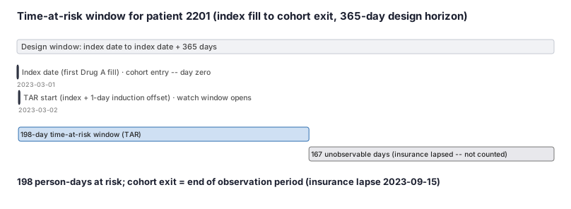
A Medicare claims study is asking whether a new blood-pressure drug (Drug A) causes a first hospitalization for heart failure. Patient 2201 fills Drug A for the first time on 2023-03-01 -- that is the index date. The study design says: open the watch window one day after the index date (to avoid counting heart failure that was already coded on the fill day), and follow each patient for up to 365 days. Patient 2201 loses insurance coverage on 2023-09-15; after that date her claims are invisible to the database. She never has a heart-failure hospitalization before that date. We want to know how many days she contributes to the study denominator and why her follow-up ends when it does.

Dataset

Key dates for patient 2201 pulled from OMOP-style tables -- the anchors an analyst joins before computing the time-at-risk window.

Steps

• Set the TAR start: add the 1-day induction offset to the index date. TAR start = 2023-03-01 + 1 day = 2023-03-02.

• Identify all possible TAR end dates: (a) design end rule = 2023-03-01 + 365 days = 2024-02-29 (leap year); (b) insurance coverage ends = 2023-09-15; (c) outcome never occurred, so no outcome exit date applies.

• Apply the 'whichever comes first' rule: compare 2024-02-29 and 2023-09-15. The earlier date is 2023-09-15.

• Cohort exit = 2023-09-15 because insurance lapse comes well before the 365-day design limit.

• Calculate days at risk: from 2023-03-02 through 2023-09-15 inclusive = 198 days.

• Record the exit reason: the patient did not have the outcome; she exited because observable follow-up ended when insurance coverage lapsed. She contributes 198 person-days to the study denominator and zero outcome events.

Result

Label

198 days at risk; cohort exit = end of observation period (insurance lapse on 2023-09-15)

Value

198

Timeline Spec

Title

Time-at-risk window for patient 2201 (index fill to cohort exit, 365-day design horizon)

Caption

The TAR window opens 1 day after the index fill and closes at insurance lapse (198 days), well before the 365-day design limit. No outcome occurred, so the patient contributes 198 person-days to the study denominator and no events to the numerator.

Alt Text

A horizontal timeline showing: index date on 2023-03-01, TAR start one day later on 2023-03-02, a blue shaded 198-day at-risk span ending at cohort exit on 2023-09-15 due to insurance lapse, and the unfulfilled design end rule shown as a dashed line extending to 2024-02-29. A grey shaded region from 2023-09-15 to 2024-02-29 is labeled unobservable.

Window

Start

2023-03-01

End

2024-02-29

Label

Design window: index date to index date + 365 days

Events

• Label

  Index date (first Drug A fill)

  Start

  2023-03-01

  Length Days

  1

  Quantity

  cohort entry -- day zero

• Label

  TAR start (index + 1-day induction offset)

  Start

  2023-03-02

  Length Days

  1

  Quantity

  watch window opens

Spans

• Kind

  followup

  Start

  2023-03-02

  End

  2023-09-15

  Label

  198-day time-at-risk window (TAR)

• Kind

  unexposed

  Start

  2023-09-16

  End

  2024-02-29

  Label

  167 unobservable days (insurance lapsed -- not counted)

Result

Label

198 person-days at risk; cohort exit = end of observation period (insurance lapse 2023-09-15)

Value

198

Runnable example

import pandas as pd

INDUCTION_OFFSET = pd.Timedelta(days=1)    # +1: exclude outcomes coded on the index day (prevalent, not incident)
ITT_HORIZON      = pd.Timedelta(days=730)  # fixed ITT follow-up horizon
GRACE            = pd.Timedelta(days=90)    # on-treatment grace after last days_supply end

def build_tar(cohort: pd.DataFrame, obs: pd.DataFrame,
              death: pd.DataFrame, drug_era: pd.DataFrame) -> pd.DataFrame:
    df = cohort.merge(obs, on="person_id", how="left") \
               .merge(death, on="person_id", how="left")

    # On-treatment era end = last drug_era_end_date for this person's index era + grace.
    era_end = (drug_era.groupby("person_id")["drug_era_end_date"].max()
                       .rename("era_end").reset_index())
    df = df.merge(era_end, on="person_id", how="left")

    # TAR start: time zero + induction offset.
    df["tar_start"] = df["cohort_start_date"] + INDUCTION_OFFSET

    # Loss-of-observability fl:  cohort exit can never exceed observed person-time.
    obs_floor = df[["observation_period_end_date", "death_date"]].min(axis=1)

    # ITT-like exit = min(fixed horizon, end of observability).
    df["tar_end_itt"] = pd.concat(
        [df["cohort_start_date"] + ITT_HORIZON, obs_floor], axis=1).min(axis=1)

    # On-treatment exit = min(era end + grace, end of observability).
    df["tar_end_ontx"] = pd.concat(
        [df["era_end"] + GRACE, obs_floor], axis=1).min(axis=1)

    # Drop persons with no positive person-time (exit on or before tar_start).
    df = df[df["tar_end_itt"] > df["tar_start"]].copy()
    return df[["person_id", "cohort_start_date", "tar_start",
               "tar_end_itt", "tar_end_ontx", "death_date"]]

library(data.table)

INDUCTION <- 1L     # +1 day induction offset (exclude index-day prevalent outcomes)
ITT_HORIZON <- 730L  # fixed ITT horizon in days
GRACE <- 90L         # on-treatment grace after last era end

build_tar <- function(cohort, obs, death, drug_era) {
  setDT(cohort); setDT(obs); setDT(death); setDT(drug_era)

  era_end <- drug_era[, .(era_end = max(drug_era_end_date)), by = person_id]

  df <- merge(cohort, obs[, .(person_id, observation_period_end_date)], by = "person_id", all.x = TRUE)
  df <- merge(df, death[, .(person_id, death_date)], by = "person_id", all.x = TRUE)
  df <- merge(df, era_end, by = "person_id", all.x = TRUE)

  df[, tar_start := cohort_start_date + INDUCTION]

  # Cohort exit can never exceed observed person-time (min of obs-period end and death).
  df[, obs_floor := pmin(observation_period_end_date, death_date, na.rm = TRUE)]

  df[, tar_end_itt  := pmin(cohort_start_date + ITT_HORIZON, obs_floor, na.rm = TRUE)]
  df[, tar_end_ontx := pmin(era_end + GRACE,               obs_floor, na.rm = TRUE)]

  df <- df[tar_end_itt > tar_start]   # require positive person-time
  df[, .(person_id, cohort_start_date, tar_start, tar_end_itt, tar_end_ontx, death_date)]
}