OMOP Drug Exposure and Drug Era

In plain language

When a patient fills a prescription, that fill gets stored as a single row in the DRUG_EXPOSURE table — one row per trip to the pharmacy, with the drug name, fill date, and how many days' worth of pills the bottle contains. A DRUG_ERA collapses those individual fills into a single continuous-treatment span: as long as a new fill arrives within a tolerance window (the default is 30 days after the previous supply runs out), the algorithm treats the patient as still on the drug and extends the episode rather than starting a new one. The era is the unit most studies use when asking 'how long was this patient on treatment' — but the 30-day tolerance is a modeling choice, not a medical fact, and changing it to 0 or 90 days can meaningfully shift who counts as 'exposed' and for how long.

In the OMOP Common Data Model (CDM), drug exposure is represented at two distinct grains, and confusing them is a common source of silent misclassification in RWE. DRUG_EXPOSURE is the atomic table: one row per source-level dispensing, prescription, or administration, keyed on `person_id` with `drug_concept_id` mapped to the standardized vocabulary at the clinical-drug level (e.g., RxNorm clinical/branded drug), plus `drug_exposure_start_date`, `drug_exposure_end_date`, `days_supply`, `quantity`, and `route_concept_id`. DRUG_ERA is a derived table: it rolls clinical drugs up to their ingredient (via `CONCEPT_ANCESTOR`), then stitches consecutive exposures of the same ingredient into a single episode (`drug_era_start_date`, `drug_era_end_date`, `gap_days`, `drug_exposure_count`) whenever the gap between the end of one exposure and the start of the next falls within a persistence threshold. The OHDSI-default persistence window is 30 days. Drug eras are the unit most analyses treat as "a treatment episode."

Core conceptual distinction

. DRUG_EXPOSURE is what the source said happened — a faithful, claim-by-claim or order-by-order ledger at the clinical-drug grain. DRUG_ERA is an analyst's model of continuous treatment at the ingredient grain, and its boundaries are an explicit, consequential parameter, not a fact in the data. Three decisions are folded into a drug era and must be pre-specified in the estimand: (1) the ingredient roll-up (a patient switching between two atorvastatin products is one statin era, but atorvastatin → rosuvastatin is two ingredient eras even though it is "continuous statin therapy"); (2) the end-date imputation when `days_supply` is missing or implausible (impute from quantity ÷ a typical daily dose, or a fixed default — this directly sets where person-time ends); and (3) the persistence gap that allows late refills to be treated as one continuous era (0, 30, 90 days). The gap is the dominant judgment call: a 0-day gap demands seamless refills and shortens person-time, treating every late refill as discontinuation; a 90-day gap forgives long supply gaps and lengthens on-treatment time, risking immortal-time-like overcounting of exposed person-time during periods the patient held no drug.

Pros, cons, and trade-offs

. - DRUG_ERA vs analyzing raw DRUG_EXPOSURE rows directly: Eras give you ready-made, ingredient-level episodes that map cleanly onto persistence, time-at-risk, and on-treatment follow-up; they absorb the messy "stockpiling / overlapping fills / one-day gaps" bookkeeping into a single transparent rule. Cost: the default 30-day era hides the gap choice from downstream users, and the ingredient roll-up erases within-class switching that may be the exposure contrast of interest. Prefer raw DRUG_EXPOSURE when you need clinical-drug-level detail (dose, formulation, brand, route) or when switching between agents in the same ingredient family is itself the exposure. - OMOP DRUG_ERA vs a bespoke claims episode-construction algorithm (e.g., PDC/MPR-style stitching outside OMOP): The OMOP era algorithm is standardized, network-portable (the same code runs across CDM sites without re-mapping), and reviewable. Cost: the standard ERA derivation is deliberately simple — it does not, by default, cap stockpiling, handle inpatient bridging, or model dynamic dosing. Prefer a bespoke or extended algorithm (or `exposure-episode-construction-rwe`) when those features change the answer, and document the deviation from the standard era. - Ingredient-level DRUG_ERA vs clinical-drug-level exposure windows: Ingredient eras are the right grain for "any statin" questions and for class-level safety; clinical-drug windows are required for dose-response, biosimilar/branded contrasts, or formulation-specific signals. They are not interchangeable, and silently using the era table for a clinical-drug question is a misclassification, not a simplification.

When to use

. Use DRUG_ERA when the analytic unit is a continuous ingredient-level treatment episode: defining new-user cohorts and washouts, building on-treatment (as-treated) follow-up, measuring persistence and time-to-discontinuation, or running ingredient-level comparative safety/effectiveness across an OHDSI network where standardization and portability matter. Use DRUG_EXPOSURE directly when you need dose, quantity, route, brand/clinical-drug identity, or when you will define your own episode logic and want full control over the gap, stockpiling, and imputation rules.

When NOT to use — and when it is actively misleading or dangerous

. - Treating the default 30-day era as a neutral fact. It is a modeling choice. Reporting "exposed person-time" off a default era without a sensitivity analysis on the gap (0/30/90) hides the parameter that most moves rates — and a too-generous gap manufactures exposed person-time during true non-use, biasing safety analyses toward the null (events accrue while the patient is unprotected but still counted as "on drug"). - Using ingredient eras for a within-ingredient or dose question. The roll-up destroys exactly the contrast you need; you will silently pool brands, doses, and formulations. - Imputing end dates from `days_supply` when `days_supply` is unreliable. In administration-based EHR data and in inpatient claims, `days_supply` is frequently missing, zero, or a placeholder. Mechanically imputing a fixed default fabricates era length and corrupts both persistence and time-at-risk; verify the `days_supply` distribution before trusting it. - Comparing eras across CDM sites that used different ERA-derivation parameters. If site A built 30-day eras and site B built 90-day eras, "drug era" is not the same variable; network analyses must pin the persistence gap and re-derive eras uniformly, never assume the vendor-shipped DRUG_ERA table is comparable.

Data-source operational depth

. - Claims (FFS pharmacy): The cleanest substrate — each adjudicated pharmacy claim is a DRUG_EXPOSURE row with a real `days_supply` and `quantity`; eras stitch well. Failure modes: claim reversals/voids must be removed before stitching or you double-count supply; 90-day mail-order and free samples distort `days_supply`; same-day duplicate fills inflate `drug_exposure_count`. Critically, Medicare Advantage (MA) enrollees lack fee-for-service pharmacy claims unless Part D encounter data are present — an MA-only person looks like "no fills," so an apparent washout or discontinuation is missingness, not non-use. Restrict era-based person-time to spans with observable pharmacy benefit (Part D / commercial Rx). - EHR: DRUG_EXPOSURE here is usually an order or administration, not a dispensing; `days_supply` is often absent for inpatient administrations and outpatient orders, forcing end-date imputation. Visit-driven capture means a patient who gets care outside the system shows phantom gaps that the era algorithm will read as discontinuation. Prefer linkage to pharmacy fills to confirm the patient actually started and continued, and treat loss to follow-up as potentially informative. - Registry: Often records treatment status or regimen rather than dispensing-level supply, so native drug eras may not be derivable at all; link to claims for the fill history before building eras, and to a death index so the era does not run past death. - Linked claims–EHR–vital records: The ideal substrate (EHR for dose/route/severity, claims for complete fills, vital records for censoring), but order/fill/administration date discrepancies must be reconciled before era stitching, and the linkable subset introduces selection.

Worked claims example

Goal: build 30-day statin drug eras and use them to define a new-user, on-treatment window. (1) Source rows (DRUG_EXPOSURE): person 1001 has pharmacy fills for atorvastatin 20 mg (NDC X) on 2023-01-05 with `days_supply` 30, a refill on 2023-02-10 (`days_supply` 30), and atorvastatin 40 mg (NDC Y) on 2023-03-20 (`days_supply` 90). (2) NDC → ingredient roll-up: both NDCs map through the standardized vocabulary to the atorvastatin ingredient via `CONCEPT_ANCESTOR`, so all three rows belong to one candidate ingredient era. (3) End-date imputation: each exposure `drug_exposure_end_date = drug_exposure_start_date + days_supply − 1`, giving covered windows [01-05 … 02-03], [02-10 … 03-11], [03-20 … 06-17]. (4) Gap-stitching walk with a 30-day persistence gap: fill 1 ends 02-03; fill 2 starts 02-10 → gap = 6 days ≤ 30 → same era. Fill 2 ends 03-11; fill 3 starts 03-20 → gap = 8 days ≤ 30 → same era. Result: one DRUG_ERA for atorvastatin, `drug_era_start_date` 2023-01-05, `drug_era_end_date` 2023-06-17, `drug_exposure_count` 3, `gap_days` 14 (total within-era gap). Had the third fill arrived on 2023-05-01 (gap = 51 days > 30), the algorithm would split it into two eras — and any safety event in late March/April would change from "on-treatment" to "post-discontinuation," a classification that flips entirely with the gap parameter. (5) Propagation to design: the new-user washout requires no atorvastatin DRUG_EXPOSURE in the 365-day lookback before `drug_era_start_date` (and continuous, FFS-observable Part D enrollment so that absence of fills is real, not MA-only missingness); on-treatment follow-up runs from the era start to `drug_era_end_date` (+ an optional grace period), censoring at disenrollment, death, end of data, or switch to a different statin ingredient. The same era boundaries feed `omop-time-at-risk-cohort-exit-rwe` and persistence (`persistence-time-to-discontinuation`); report rates under 0-, 30-, and 90-day gaps as the primary sensitivity analysis.

Worked example

Scenario

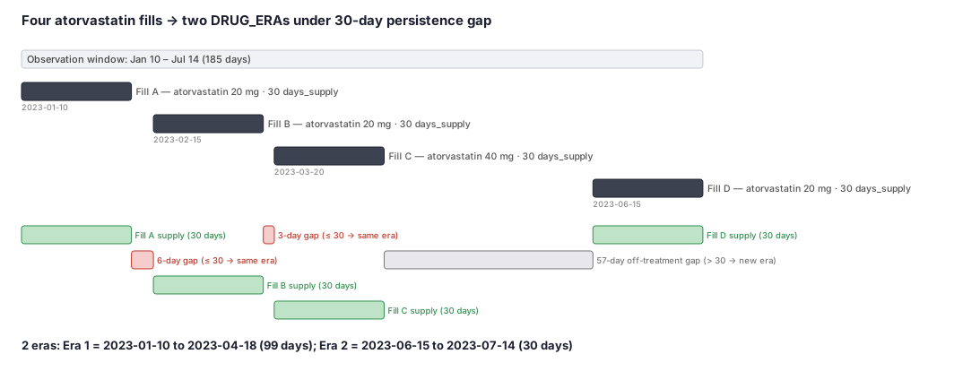
Person 1001 fills atorvastatin — a cholesterol-lowering drug — four times over about seven months. We want to know how many continuous treatment episodes the OMOP algorithm would build from those four fills using the default 30-day persistence gap. Each fill covers exactly as many days as its days_supply; when a new fill arrives within 30 days after the previous supply would run out, it is stitched onto the same era. If the gap exceeds 30 days, a new era begins. Both atorvastatin 20 mg and atorvastatin 40 mg roll up to the same 'atorvastatin' ingredient, so all four fills are candidates for the same era.

Dataset

Raw DRUG_EXPOSURE rows for person 1001 — exactly what an analyst would see in the OMOP pharmacy table.

Steps

• Each fill's end date is fill_date + days_supply − 1: Fill A ends Feb 8, Fill B ends Mar 16, Fill C ends Apr 18, Fill D ends Jul 14.

• Gap A→B: Fill A supply runs out Feb 8; Fill B arrives Feb 15 — that is 6 days later. 6 ≤ 30, so Fill B is stitched onto Era 1.

• Gap B→C: Fill B supply runs out Mar 16; Fill C arrives Mar 20 — that is 3 days later. 3 ≤ 30, so Fill C is stitched onto Era 1.

• Era 1 now spans Jan 10 through Apr 18 (the latest end date among Fills A, B, C), covering 99 calendar days with 90 days of actual supply and 9 days of within-era gap (6 + 3).

• Gap C→D: Fill C supply runs out Apr 18; Fill D arrives Jun 15 — that is 57 days later. 57 > 30, so the algorithm closes Era 1 and opens Era 2 at Fill D.

• Era 2 contains only Fill D: Jun 15 through Jul 14, covering exactly 30 days with 0 within-era gap.

Result

Label

2 drug eras: Era 1 spans 2023-01-10 to 2023-04-18 (99 days, 3 fills, 9 within-era gap days); Era 2 spans 2023-06-15 to 2023-07-14 (30 days, 1 fill, 0 gap days). Any outcome event in the 57-day window between Apr 19 and Jun 14 is off-treatment under the 30-day gap rule.

Value

Era Count

2

Era 1 Length Days

99

Era 2 Length Days

30

Timeline Spec

Title

Four atorvastatin fills → two DRUG_ERAs under 30-day persistence gap

Caption

Fills A, B, and C are separated by gaps of 6 and 3 days (both within the 30-day threshold) and merge into Era 1. Fill D arrives 57 days after Fill C's supply ends — exceeding the threshold — so it opens Era 2. Any event in the 57-day off-treatment window between Era 1 and Era 2 is classified as post-discontinuation, not on-treatment.

Alt Text

Timeline showing four prescription fill bars labeled Fill A through Fill D. Fill A (Jan 10–Feb 8), Fill B (Feb 15–Mar 16), and Fill C (Mar 20–Apr 18) are bridged by a shaded Era 1 span with two small gap bands of 6 and 3 days. A wide off-treatment gap band stretches from Apr 19 to Jun 14 (57 days). Fill D (Jun 15–Jul 14) sits alone under a shaded Era 2 span.

Window

Start

2023-01-10

End

2023-07-14

Label

Observation window: Jan 10 – Jul 14 (185 days)

Events

• Label

  Fill A — atorvastatin 20 mg

  Start

  2023-01-10

  Length Days

  30

  Quantity

  30 days_supply

• Label

  Fill B — atorvastatin 20 mg

  Start

  2023-02-15

  Length Days

  30

  Quantity

  30 days_supply

• Label

  Fill C — atorvastatin 40 mg

  Start

  2023-03-20

  Length Days

  30

  Quantity

  30 days_supply

• Label

  Fill D — atorvastatin 20 mg

  Start

  2023-06-15

  Length Days

  30

  Quantity

  30 days_supply

Spans

• Kind

  exposed

  Start

  2023-01-10

  End

  2023-02-08

  Label

  Fill A supply (30 days)

• Kind

  gap

  Start

  2023-02-09

  End

  2023-02-14

  Label

  6-day gap (≤ 30 → same era)

• Kind

  exposed

  Start

  2023-02-15

  End

  2023-03-16

  Label

  Fill B supply (30 days)

• Kind

  gap

  Start

  2023-03-17

  End

  2023-03-19

  Label

  3-day gap (≤ 30 → same era)

• Kind

  exposed

  Start

  2023-03-20

  End

  2023-04-18

  Label

  Fill C supply (30 days)

• Kind

  unexposed

  Start

  2023-04-19

  End

  2023-06-14

  Label

  57-day off-treatment gap (> 30 → new era)

• Kind

  exposed

  Start

  2023-06-15

  End

  2023-07-14

  Label

  Fill D supply (30 days)

Result

Label

2 eras: Era 1 = 2023-01-10 to 2023-04-18 (99 days); Era 2 = 2023-06-15 to 2023-07-14 (30 days)

Value

Era Count

2

Era 1 Length Days

99

Era 2 Length Days

30

Runnable example

import pandas as pd
import numpy as np

PERSISTENCE_GAP = 30  # days a refill may be late before a new era starts; sensitivity-test 0 / 30 / 90

def build_drug_eras(drug_exposure: pd.DataFrame,
                    concept_ancestor: pd.DataFrame,
                    gap_days: int = PERSISTENCE_GAP) -> pd.DataFrame:
    de = drug_exposure.copy()

    # Roll clinical drugs up to their ingredient via CONCEPT_ANCESTOR.
    anc = concept_ancestor.rename(columns={"descendant_concept_id": "drug_concept_id",
                                           "ancestor_concept_id": "ingredient_concept_id"})
    de = de.merge(anc[["drug_concept_id", "ingredient_concept_id"]], on="drug_concept_id", how="inner")

    # Impute end date from days_supply when missing (start + days_supply - 1).
    need = de["drug_exposure_end_date"].isna()
    de.loc[need, "drug_exposure_end_date"] = (
        de.loc[need, "drug_exposure_start_date"]
        + pd.to_timedelta(de.loc[need, "days_supply"].fillna(0).astype(int) - 1, unit="D"))

    de = de.sort_values(["person_id", "ingredient_concept_id", "drug_exposure_start_date"])

    # Carry-over: a new era starts when the current fill begins more than gap_days after the
    # running maximum covered end date for this (person, ingredient). cummax handles overlap/stockpiling.
    g = de.groupby(["person_id", "ingredient_concept_id"], sort=False)
    prev_cov_end = g["drug_exposure_end_date"].cummax().groupby(
        [de["person_id"], de["ingredient_concept_id"]]).shift()
    gap = (de["drug_exposure_start_date"] - prev_cov_end).dt.days
    new_era = prev_cov_end.isna() | (gap > gap_days)
    de["era_id"] = new_era.groupby([de["person_id"], de["ingredient_concept_id"]]).cumsum()

    eras = (de.groupby(["person_id", "ingredient_concept_id", "era_id"])
              .agg(drug_era_start_date=("drug_exposure_start_date", "min"),
                   drug_era_end_date=("drug_exposure_end_date", "max"),
                   drug_exposure_count=("drug_concept_id", "size"),
                   covered_days=("days_supply", "sum"))
              .reset_index())
    # gap_days = elapsed span not covered by supply within the era.
    span = (eras["drug_era_end_date"] - eras["drug_era_start_date"]).dt.days + 1
    eras["gap_days"] = (span - eras["covered_days"]).clip(lower=0)
    return eras.drop(columns="covered_days")

library(data.table)
PERSISTENCE_GAP <- 30L  # sensitivity-test 0 / 30 / 90

build_drug_eras <- function(drug_exposure, concept_ancestor, gap_days = PERSISTENCE_GAP) {
  de  <- as.data.table(drug_exposure)
  anc <- as.data.table(concept_ancestor)[, .(drug_concept_id = descendant_concept_id,
                                             ingredient_concept_id = ancestor_concept_id)]
  de <- merge(de, anc, by = "drug_concept_id", allow.cartesian = TRUE)

  # Impute missing end date from days_supply.
  de[is.na(drug_exposure_end_date),
     drug_exposure_end_date := drug_exposure_start_date + as.integer(fifelse(is.na(days_supply), 0L, days_supply)) - 1L]

  setorder(de, person_id, ingredient_concept_id, drug_exposure_start_date)

  # Running max covered end date (cummax) per person-ingredient handles overlap/stockpiling.
  de[, prev_cov_end := shift(cummax(as.integer(drug_exposure_end_date))),
     by = .(person_id, ingredient_concept_id)]
  de[, gap := as.integer(drug_exposure_start_date) - prev_cov_end]
  de[, new_era := is.na(prev_cov_end) | gap > gap_days]
  de[, era_id := cumsum(new_era), by = .(person_id, ingredient_concept_id)]

  eras <- de[, .(drug_era_start_date  = min(drug_exposure_start_date),
                 drug_era_end_date    = max(drug_exposure_end_date),
                 drug_exposure_count  = .N,
                 covered_days         = sum(days_supply, na.rm = TRUE)),
             by = .(person_id, ingredient_concept_id, era_id)]
  eras[, gap_days := pmax(0L, as.integer(drug_era_end_date - drug_era_start_date) + 1L - covered_days)]
  eras[, covered_days := NULL][]
}