OMOP Observation Period

In plain language

An OMOP Observation Period is the recorded span of time during which a data source can actually see a patient — their health insurance was active, they were visiting the clinic, or they were enrolled in a registry. Any clinical event that happens outside this window is simply invisible to the database: the absence of a record there means nothing, because no one was watching. Every study built on OMOP data must anchor its lookback and its follow-up windows inside this observable span, or the researcher risks counting missing data as evidence that events never happened.

The OMOP `observation_period` table is the CDM's formal answer to a question every real-world study must answer before any exposure, covariate, or outcome is counted: when was this person actually under observation in this data source? Each row is a `[observation_period_start_date, observation_period_end_date]` span for a `person_id`, tagged with a `period_type_concept_id` describing how the span was derived (e.g., from enrollment files in claims, from the first/last recorded clinical event in EHR). Person-time outside any observation period is unobservable, not "event-free": the absence of a diagnosis, fill, or procedure there is missingness, not evidence of non-occurrence. Every defensible OMOP study therefore anchors its lookback (baseline) window and its at-risk (follow-up) window inside observation-period spans.

Core conceptual distinction

. The observation period is the substrate of observability, distinct from three things it is routinely confused with. (1) It is not the cohort time-at-risk: time-at-risk is a study-defined window (index date plus a risk-window rule), whereas the observation period is the source-level envelope that the time-at-risk must fit within. (2) It is not continuous enrollment per se: in an ETL'd claims source the two often coincide because the period is built from enrollment spans, but in EHR the period is inferred from clinical-activity boundaries and a person can be "enrolled" yet invisible (no encounters). (3) It is not the washout/lookback rule: washout is an exposure-cleaning decision applied within observable time; the observation period determines whether enough observable time exists to evaluate the washout at all. The downstream consequence is concrete: requiring `observation_period_start_date <= index_date - lookback_days` makes "no prior diagnosis/fill" a true absence; requiring `observation_period_end_date >= index_date + min_followup` prevents counting people who were never observable long enough to experience the outcome.

Pros, cons, and trade-offs

- vs ad-hoc continuous-enrollment flags built directly from raw enrollment claims: The OMOP `observation_period` is a single, ETL-validated, source-agnostic abstraction, so the same OHDSI cohort/PLP/PLE code runs unchanged across claims, EHR, and registry data and across a federated network. Cost: the ETL's gap-collapsing rules (how many days of no enrollment break a period; whether short gaps are bridged) are baked in upstream and may not match your protocol — you inherit decisions you did not make. Prefer the CDM table for network/portable studies; prefer raw enrollment spans when you need bespoke gap rules and control the analysis end-to-end. - vs ignoring observability (using all recorded events): Anchoring to observation periods removes left-truncation bias (treating a prevalent condition recorded on day 1 of data as incident) and removes spurious "event-free" person-time. Cost: cohort size shrinks and the surviving population skews toward the continuously observable, who differ from the transient population. Always prefer observability-anchored analysis; the alternative is not a trade-off, it is a bug. - vs a single global lookback applied uniformly: Using `observation_period_start_date` to define an all-available lookback captures more comorbidity history but makes covariate ascertainment depend on observable duration (people seen longer accrue more codes), inducing differential measurement by exposure if observable time differs across arms. A fixed lookback (e.g., 365 days, requiring the period to cover it) standardizes ascertainment at the cost of discarding short-history patients. Prefer a fixed, enforced lookback for comparative analyses; reserve all-available lookback for prediction, where calibration tolerates it.

When to use

. Any study built on the OMOP CDM: defining cohort eligibility (require observable lookback and follow-up), bounding time-at-risk so follow-up never extends past `observation_period_end_date`, computing incidence-rate denominators from observable person-time, and ensuring portability of a protocol across a federated OHDSI network where each site's observability is encoded the same way. It is the gatekeeper step that runs before exposure and outcome logic.

When NOT to use — and when it is actively misleading or dangerous

. It is dangerous to treat the observation period as a clinical truth rather than a data-capture artifact. (1) EHR end-dates as outcome ascertainment: an `observation_period_end_date` derived from "last recorded event" can be set by the outcome itself — a patient who dies or becomes too sick to visit simply stops generating records, so censoring at the period end can censor on the outcome, biasing rates downward. Use an external death index, do not infer end-of-observability from clinical silence. (2) Mistaking a payer-driven period boundary for a clinical event: disenrollment is administrative; ending follow-up there is correct for observability but must not be read as "the patient was stable." (3) All-available lookback in a comparative study when observable duration differs by arm — it manufactures differential confounder measurement. (4) Single-period assumptions when the source allows multiple periods per person: silently using only the first (or only the longest) period drops valid follow-up and can break the requirement that index falls inside an observable span.

Data-source operational depth

- Claims (FFS): `observation_period` is typically ETL'd from medical+pharmacy enrollment spans. The ETL's gap rule matters: short administrative gaps may be bridged into one period or split into several; verify the rule before requiring "continuous" lookback. Failure mode: Medicare Advantage person-time is frequently absent from FFS claims, so an MA enrollee can have an observation period reflecting only their FFS months — apparent "gaps" or short periods are MA capitation, not true unobservability. Restrict to FFS Parts A/B/D (or the equivalent commercial medical+pharmacy benefit) and exclude MA-only spans rather than trusting the period blindly. - EHR: `observation_period` is usually inferred from the first to last clinical event (visits, labs, orders). This makes the boundaries encounter-driven and informatively censored: sicker, frequently-seen patients have long dense periods; healthy or transient patients have short sparse ones, and external care leakage (care delivered outside the health system) is invisible inside the period. Differential follow-up by exposure is the rule, not the exception; treat `observation_period_end_date` as potentially outcome-dependent and supplement with linked mortality. - Registry: Observability is enrollment in the registry plus its ascertainment completeness; the OMOP period (if the registry is mapped) reflects registry contact, not full healthcare exposure. Link to claims for complete drug/utilization person-time and to a death index for censoring. - Linked claims–EHR–vital records: The richest substrate, but each source contributes its own observation periods with different `period_type_concept_id` values and different boundary semantics. Reconcile them explicitly (intersection for "observable everywhere," union for "observable somewhere") before defining lookback/follow-up; never pool periods of different types as if interchangeable, and watch for differential competing risks (e.g., death censoring observable time more in the older/sicker arm).

Worked claims example

Question: 12-month incidence of acute kidney injury (AKI) after initiating a study drug among adults, in an OMOP-mapped commercial + Medicare FFS source that allows multiple observation periods per person (payer changes split spans). Setup: cohort entry (`index_date`) = first qualifying `drug_exposure` start; lookback = 365 days; minimum follow-up to be evaluable = none (rate analysis uses observable person-time), but follow-up is censored at the earliest of AKI, `observation_period_end_date`, death, or 365 days post-index. Steps: (1) For each candidate `index_date`, find the single observation period that contains the index date — not the first, not the longest — because exposure and follow-up must live inside one contiguous observable span. (2) Eligibility lookback: keep the person only if that containing period satisfies `observation_period_start_date <= index_date - 365`, so "no prior AKI / no prior study drug" in the baseline window reflects true absence rather than an unobserved gap. (3) Restrict `period_type_concept_id` to the claims-enrollment-derived type and exclude MA-only spans, so a short period is not mistaken FFS for capitated MA time. (4) At-risk window: `risk_start = index_date`, `risk_end = min(index_date + 365, observation_period_end_date, death_date)`; observable person-time for the rate denominator is `risk_end - risk_start`, never extending past the period end. (5) Count the first AKI `condition_occurrence` whose date lies inside the at-risk window. (6) Diagnostics before trusting anything: distribution of observable lookback and follow-up days by arm (differential observability is a confounding-measurement red flag), count of persons with >1 observation period, and a sensitivity analysis varying the lookback requirement (e.g., 183 vs 365 days) and the gap-bridging assumption. The single highest-yield check is plotting follow-up length by exposure arm: if the curves separate, your `observation_period_end_date` is encoding something exposure-related and a naive rate is biased.

Worked example

Scenario

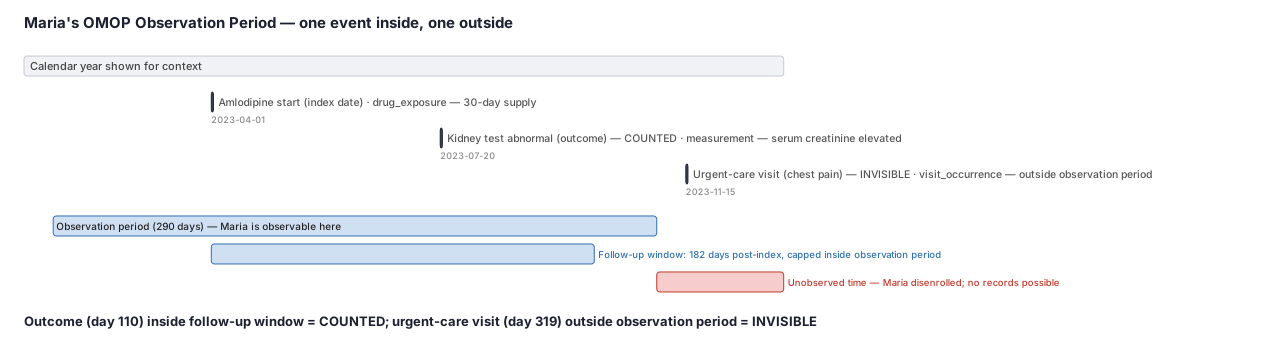
Maria is a 58-year-old patient in a commercial claims database. Her insurer enrolled her on 2023-01-15 and she disenrolled on 2023-10-31, giving her a single observation period of 290 days. A researcher wants to study whether a new blood-pressure drug (amlodipine) is associated with a kidney function test abnormality within 6 months of starting the drug. Maria started amlodipine on 2023-04-01 and had a kidney test come back abnormal on 2023-07-20 — both fall inside her observation period. She also had an urgent-care visit for chest pain on 2023-11-15 — but she had already disenrolled, so that visit is completely invisible to the database.

Dataset

The OMOP observation_period table row for Maria, plus her two clinical events.

Steps

• Identify Maria's observation period: 2023-01-15 through 2023-10-31 (290 days).

• Confirm the index date (amlodipine start, 2023-04-01) falls inside the observation period — it does (day 76 of 290).

• Check the lookback window: to verify Maria had no prior kidney problems, the researcher needs at least 90 days before 2023-04-01, meaning back to 2023-01-01. Her observation period starts 2023-01-15, so only 76 days of clean lookback are available — the researcher must decide whether that is sufficient or must exclude Maria.

• Set the follow-up window: the researcher wants 6 months (182 days) after 2023-04-01, which would end 2023-10-01. That date is before the observation period end (2023-10-31), so the full 6-month follow-up is observable.

• Find outcomes inside the follow-up: the kidney test on 2023-07-20 falls between 2023-04-01 and 2023-10-01 — it is counted as the event.

• The urgent-care visit on 2023-11-15 is 15 days after the observation period ends — the database has no record of it, so the researcher cannot see or count it.

• Result: Maria contributed 182 observable follow-up days and had one outcome event on day 110.

Result

Label

Observable follow-up days / outcome found inside window

Value

182 follow-up days (2023-04-01 to 2023-10-01); outcome on day 110 (2023-07-20); post-period event on 2023-11-15 is unobserved and not counted

Timeline Spec

Title

Maria's OMOP Observation Period — one event inside, one outside

Window

Start

2023-01-01

End

2023-12-31

Label

Calendar year shown for context

Events

• Label

  Amlodipine start (index date)

  Start

  2023-04-01

  Length Days

  1

  Quantity

  drug_exposure — 30-day supply

• Label

  Kidney test abnormal (outcome) — COUNTED

  Start

  2023-07-20

  Length Days

  1

  Quantity

  measurement — serum creatinine elevated

• Label

  Urgent-care visit (chest pain) — INVISIBLE

  Start

  2023-11-15

  Length Days

  1

  Quantity

  visit_occurrence — outside observation period

Spans

• Kind

  followup

  Start

  2023-01-15

  End

  2023-10-31

  Label

  Observation period (290 days) — Maria is observable here

• Kind

  followup

  Start

  2023-04-01

  End

  2023-10-01

  Label

  Follow-up window: 182 days post-index, capped inside observation period

• Kind

  gap

  Start

  2023-11-01

  End

  2023-12-31

  Label

  Unobserved time — Maria disenrolled; no records possible

Result

Label

Outcome (day 110) inside follow-up window = COUNTED; urgent-care visit (day 319) outside observation period = INVISIBLE

Value

1 outcome event observed; 1 event unobserved

Caption

Maria's 290-day observation period runs from her insurance enrollment (2023-01-15) to disenrollment (2023-10-31). Her amlodipine start and subsequent kidney test both fall inside this window and are counted. Her urgent-care visit 15 days after disenrollment is invisible to the database — not event-free, just unobserved.

Alt Text

A horizontal timeline spanning 2023. A blue bar labeled 'Observation period (290 days)' runs from January 15 to October 31. Inside it, two point events are marked: 'Amlodipine start (index date)' on April 1 and 'Kidney test abnormal — COUNTED' on July 20. A shaded follow-up bar runs from April 1 to October 1 (182 days). After October 31, a gray shaded region labeled 'Unobserved time' extends to December 31, with a point event 'Urgent-care visit — INVISIBLE' marked on November 15 inside the gray zone.

Runnable example

import pandas as pd

LOOKBACK_DAYS = 365     # required observable baseline before index
MAX_FOLLOWUP  = 365     # cap the at-risk window post-index
CLAIMS_TYPES  = {44814724}  # period_type_concept_id for claims/enrollment-derived periods (set per source)

def anchor_to_observation_period(cohort: pd.DataFrame, obsper: pd.DataFrame) -> pd.DataFrame:
    op = obsper[obsper["period_type_concept_id"].isin(CLAIMS_TYPES)]

    # Join every candidate index to ALL of that person's periods, then keep the ONE containing the index date.
    # (Sources may record multiple periods per person; first/longest selection is a common, silent bug.)
    m = cohort.merge(op, on="person_id", how="inner")
    contains = ((m["observation_period_start_date"] <= m["index_date"]) &
                (m["observation_period_end_date"]   >= m["index_date"]))
    m = m[contains].copy()

    # Enforced fixed lookback: the containing period must start early enough that "no prior X" is a true absence.
    lookback_ok = m["observation_period_start_date"] <= m["index_date"] - pd.Timedelta(days=LOOKBACK_DAYS)
    m = m[lookback_ok].copy()

    # At-risk window bounded by observability: follow-up never extends past the period end.
    m["baseline_start"] = m["index_date"] - pd.Timedelta(days=LOOKBACK_DAYS)
    m["risk_start"]     = m["index_date"]
    m["risk_end"]       = m[["observation_period_end_date"]].assign(
                              cap=m["index_date"] + pd.Timedelta(days=MAX_FOLLOWUP)
                          ).min(axis=1)
    m["followup_days"]  = (m["risk_end"] - m["risk_start"]).dt.days

    # One contiguous evaluable span per person (drop index dates that fell in inter-period gaps: none survive 'contains').
    return (m.sort_values(["person_id", "index_date"])
             .drop_duplicates("person_id")
             [["person_id", "index_date", "baseline_start", "risk_start", "risk_end", "followup_days"]])

library(data.table)
LOOKBACK_DAYS <- 365L
MAX_FOLLOWUP  <- 365L
CLAIMS_TYPES  <- c(44814724L)  # period_type_concept_id for claims/enrollment-derived periods (set per source)

anchor_to_observation_period <- function(cohort, obsper) {
  setDT(cohort); setDT(obsper)
  op <- obsper[period_type_concept_id %in% CLAIMS_TYPES]

  m <- merge(cohort, op, by = "person_id", allow.cartesian = TRUE)

  # Keep the observation period that CONTAINS the index date (not the first or longest one).
  m <- m[observation_period_start_date <= index_date &
         observation_period_end_date   >= index_date]

  # Enforced fixed lookback so baseline "no prior X" reflects true absence, not an unobserved gap.
  m <- m[observation_period_start_date <= index_date - LOOKBACK_DAYS]

  # At-risk window bounded by observability: follow-up cannot exceed the period end.
  m[, baseline_start := index_date - LOOKBACK_DAYS]
  m[, risk_start     := index_date]
  m[, risk_end       := pmin(observation_period_end_date, index_date + MAX_FOLLOWUP)]
  m[, followup_days  := as.integer(risk_end - risk_start)]

  setorder(m, person_id, index_date)
  unique(m, by = "person_id")[, .(person_id, index_date, baseline_start,
                                  risk_start, risk_end, followup_days)]
}