Incidence Rate Calculation

In plain language

An incidence rate counts how many new events happened and divides that by the total time the people in your study were actually being watched and could still have the event. The bottom of the fraction is not a head-count of patients; it is the summed-up time each person was followed (call it the at-risk clock), so someone watched for two years counts twice as much as someone watched for one. You report it as something like "3.7 first heart-failure hospitalizations per 1,000 person-years." The whole job is getting that at-risk clock right: stop counting a person's time the moment they have the event, leave the study, or die, because counting time they were no longer at risk quietly makes the rate look lower than it really is.

An incidence rate (IR) is events divided by person-time at risk: IR = D / PT, where D is the count of qualifying events and PT is the summed time during which each person was both observable and eligible to have a first (or next) countable event. It is a dynamic measure with units of events per person-time (e.g., per 1,000 person-years, PY) and an instantaneous-hazard interpretation — unlike a cumulative incidence (risk), which is a unitless proportion over a fixed horizon. In real-world data the IR is rarely "wrong" because of the arithmetic; it is wrong because the denominator is built from person-time that the person was not actually at risk for, or the numerator counts events the design did not intend to count. Getting the at-risk clock right is the entire job.

Core conceptual distinction

Three choices must be pre-specified in the estimand and they are separable. (1) First-event vs recurrent rate: a first-event IR removes each person from the denominator at their first event (PT accrues only until the first event); a recurrent-event IR keeps accruing PT and counts subsequent events, which requires a washout/refractory rule between events and a variance estimator that respects within-person clustering (e.g., robust/Andersen-Gill). (2) At-risk definition: PT must be intersected with the windows in which the event is biologically and administratively possible (continuously observed, not already post-event for a first-event rate, not during an exclusion window). (3) Competing events: when death (or another terminal event) precludes the outcome, the cause-specific hazard rate (censor at the competing event) and the subdistribution/cumulative incidence answer different questions — a naive cause-specific IR is fine as a rate but does not translate into the risk a patient experiences when the competing event is common. Reporting a cause-specific IR and then narrating it as a "risk" is the most frequent interpretive error.

Pros, cons, and trade-offs

- vs cumulative incidence / risk (`cumulative-incidence-risk-rwe`): The IR uses all person-time, handles staggered entry and variable follow-up natively, and is the right summary when follow-up is censored or heterogeneous. Cost: it assumes a roughly constant hazard within the window it summarizes; if the hazard is strongly time-varying (e.g., a peri-procedural spike), a single IR averages over it and misleads. Prefer the IR for sparse events with variable follow-up; prefer cumulative incidence when a fixed-horizon, patient-facing probability is the question and competing risks are non-trivial. - vs crude proportion (cases / N enrolled): A proportion ignores differential follow-up and inflates or deflates with administrative censoring; the IR is unbiased for the hazard under non-informative censoring. Cost: more programming and a correct at-risk clock. Prefer the IR whenever follow-up length differs across people, which is nearly always true in claims. - vs standardized rates (`direct-standardization-rwe`, `indirect-standardization-smr-sir-rwe`): A crude IR is fine for a single homogeneous group; comparing crude IRs across populations with different age/sex/comorbidity mixes is confounded. Direct/indirect standardization or a Poisson model with an offset removes that. Prefer standardization or modeling for any cross-group comparison; reserve the crude IR for within-stratum description.

When to use

Describing the occurrence of a new-onset outcome (incident MI, first HF hospitalization, first malignancy) in a cohort with staggered entry and censoring; computing background/expected rates for safety signal detection (observed-vs-expected); building the event counts and offsets that feed a Poisson/negative-binomial rate model; reporting per-1,000-PY rates with exact Poisson confidence intervals in a regulatory or HTA dossier.

When NOT to use — and when it is actively misleading or dangerous

- The hazard is far from constant over the summary window. A single IR over 5 years that lumps a sharp early peri-exposure spike with a flat tail is uninterpretable; either split person-time into clinically meaningful intervals (piecewise rates) or model time explicitly. Quoting one IR here is actively misleading. - Competing risks are common and you narrate the rate as a risk. In an elderly or oncology cohort where death is frequent, a cause-specific IR for a non-fatal outcome does not equal the probability a patient experiences it; converting it to a "risk" overstates patient-facing probability. Switch to a cumulative incidence function (see `competing-risks-cause-specific-fine-gray-rwe`). - Person-time includes time the person was not observable or not at risk. Counting follow-up after disenrollment, after the first event in a first-event rate, or during MA-only spans where claims are absent fabricates denominator and biases the IR downward. This is the claims analogue of immortal-time bias (see `immortal-time-bias-handling`). - Recurrent events counted as if independent. Treating multiple events per person as independent Poisson observations understates variance and produces falsely narrow CIs; use robust/clustered variance.

Data-source operational depth

- Claims (FFS): PT is the intersection of continuous medical enrollment with the at-risk window; the event date is the service/admission date of the first qualifying diagnosis (with code position and care setting specified — inpatient primary dx is more specific than any-position outpatient). Failure modes: Medicare Advantage enrollees generate no fee-for-service claims, so MA-only person-time is unobserved — including it in the denominator silently inflates PT and deflates the IR; restrict to Parts A/B (and D if drug exposure matters) and drop MA-only spans. Enrollment gaps, claims-adjudication lag near the data cut, and same-day duplicate/reversed claims all distort counts. - EHR: Event ascertainment is encounter-driven, so a patient who seeks care elsewhere ("leakage") contributes apparent event-free person-time that is actually unobserved — differential leakage by exposure biases the IR. Define an explicit "active in system" requirement (e.g., ≥1 encounter per year) and treat loss to follow-up as potentially informative; structured problem-list/lab capture sharpens the case definition over claims. - Registry: Strong for adjudicated incident events (e.g., cancer registry first primaries) but typically lacks complete follow-up for censoring; link to claims for enrollment/death to build correct person-time, and check registry completeness and reporting lag by calendar year. - Linked claims–EHR–vital records: The ideal substrate — EHR specificity + claims completeness + a death index that makes the competing-risk denominator honest. Cost: linkage selects the linkable subset, and order/service/registry date discrepancies must be reconciled before assigning event dates and closing person-time.

Worked claims example

Question: incidence rate of first hospitalized heart failure (HF) among adult new initiators of a drug in a commercial + Medicare FFS database, 2019–2023, per 1,000 PY. (1) Eligibility and clock start: index date = first qualifying fill; require 365 days of continuous medical + pharmacy enrollment before index (FFS-observable, no MA-only spans) and no prior HF diagnosis in that 365-day washout — this makes the event incident, not prevalent. (2) At-risk window start: person-time begins the day after index. (3) Event: first inpatient claim with HF as the principal diagnosis (a more specific definition than any-position outpatient); the event date is the admission date. (4) Censoring / clock stop: person-time ends at the earliest of first HF event, disenrollment, death, end of study (2023-12-31), or — because death is a competing event — we report the cause-specific rate censoring at death and separately a cumulative incidence function so the rate is not misread as a risk. (5) Denominator construction: for each person, PT = (min(stop dates) − at-risk start) in years, summing only continuous FFS-observed time and stopping at the first event (first-event rate). (6) Worked numbers: suppose 47 first HF hospitalizations accrue over 12,840 person-years. IR = 47 / 12,840 = 0.00366 per PY = 3.66 per 1,000 PY. An exact (Poisson) 95% CI uses the gamma/chi-square inversion on the count: lower = 0.5·χ²(0.025, 2·47)/12.840, upper = 0.5·χ²(0.975, 2·48)/12.840, giving roughly 2.69–4.87 per 1,000 PY. (7) Sensitivity: re-run with an any-position outpatient+inpatient HF definition, with the competing-risk death handled as a subdistribution event, and with a stricter 730-day enrollment/washout, and confirm the IR and its CI move only modestly.

Interpreting the output

An incidence rate calculation returns: 20.0 per 1,000 person-years (95% CI 14.8–26.6 per 1,000 PY) from 47 events over 2,350 person-years of follow-up.

Formal interpretation. The incidence rate is a rate, not a risk: it expresses the number of new events per unit of person-time and can theoretically exceed 1.0 when expressed as a raw fraction (hence the per-1,000 PY rescaling). The exact Poisson 95% CI is derived from the gamma distribution on the event count, not from the normal approximation, and is the appropriate interval when counts are modest. The rate is cause-specific: patients who die from a competing cause are censored at that point, so the denominator includes their at-risk time only up to the competing event. Where competing mortality differs by group, a cause-specific IR alone is insufficient to describe absolute disease burden — pair it with a cumulative incidence function estimated by Aalen-Johansen.

Practical interpretation. The 20 per 1,000 PY rate means that, on average, 2 events are expected per 100 fully observed patient-years of follow-up — not that any individual has a 2% risk by 12 months. Converting to 1-year risk requires a monotone transformation (1 − exp(−rate × time)) under a constant-rate assumption. In populations with heavy competing risks or variable follow-up, the IR and the 12-month cumulative incidence may diverge substantially; both should be reported to give a complete epidemiological picture.

Worked example

Scenario

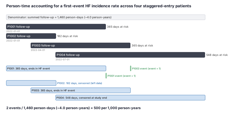
We follow four adults who just started a drug and want the incidence rate of their first hospitalized heart failure (HF) over a 2022-2023 observation window. Each person enters on a different date (staggered entry) and is followed until the earliest of their first HF hospitalization, leaving the data, or the study end on 2023-12-31. We add up everyone's follow-up time to build the denominator, count the HF events for the numerator, and divide.

Dataset

One row per patient: when their at-risk clock started, when it stopped, the resulting follow-up length, and whether the stop was an HF event (1) or a censoring (0).

Steps

• Find each person's follow-up time = exit_date minus entry_date in days: P1001 = 365, P1002 = 182, P1003 = 365, P1004 = 548 days.

• P1001 and P1003 stop because of an HF event (event = 1); P1002 stops early because they left the data and P1004 stops at the study end (both event = 0, censored), so their clocks just freeze where they are.

• Add up all the follow-up time to get total person-time: 365 + 182 + 365 + 548 = 1,460 person-days, which is 1,460 / 365 = about 4.0 person-years.

• Count the events for the numerator: 2 HF hospitalizations (P1001 and P1003).

• Divide events by total person-time, then rescale to a friendly denominator like 1,000 person-years.

Result

IR = 2 events / 1,460 person-days = 2 / 4.0 person-years = 0.50 events per person-year = 500 per 1,000 person-years. (That number is sky-high only because this teaching cohort has just 4 people followed briefly; a real HF rate from thousands of patients lands nearer 3-4 per 1,000 person-years. The mechanics of summing person-time and dividing are identical at any size.)

Timeline Spec

Title

Person-time accounting for a first-event HF incidence rate across four staggered-entry patients

Window

Start

2022-01-01

End

2023-12-31

Label

Denominator: summed follow-up = 1,460 person-days (~4.0 person-years)

Events

• Label

  P1001 follow-up

  Start

  2022-01-01

  Length Days

  365

  Quantity

  365 days at risk

• Label

  P1002 follow-up

  Start

  2022-01-01

  Length Days

  182

  Quantity

  182 days at risk

• Label

  P1003 follow-up

  Start

  2022-04-01

  Length Days

  365

  Quantity

  365 days at risk

• Label

  P1004 follow-up

  Start

  2022-07-01

  Length Days

  548

  Quantity

  548 days at risk

Spans

• Kind

  followup

  Start

  2022-01-01

  End

  2023-01-01

  Label

  P1001: 365 days, ends in HF event

• Kind

  exposed

  Start

  2023-01-01

  End

  2023-01-01

  Label

  P1001 event (event = 1)

• Kind

  followup

  Start

  2022-01-01

  End

  2022-07-02

  Label

  P1002: 182 days, censored (left data)

• Kind

  followup

  Start

  2022-04-01

  End

  2023-04-01

  Label

  P1003: 365 days, ends in HF event

• Kind

  exposed

  Start

  2023-04-01

  End

  2023-04-01

  Label

  P1003 event (event = 1)

• Kind

  followup

  Start

  2022-07-01

  End

  2023-12-31

  Label

  P1004: 548 days, censored at study end

Result

Label

2 events / 1,460 person-days (~4.0 person-years) = 500 per 1,000 person-years

Value

500.0

Caption

Four patients enter on different dates and each contributes a follow-up bar; P1001 and P1003 end in an HF event (numerator = 2), while P1002 and P1004 are censored. The four bar lengths (365 + 182 + 365 + 548 = 1,460 person-days) are the denominator the rate divides into.

Alt Text

Timeline over 2022-2023 showing four horizontal follow-up bars of 365, 182, 365, and 548 days starting on different dates; two bars (P1001, P1003) end in an event marker and two (P1002, P1004) end censored, with the summed person-time of 1,460 person-days forming the rate denominator.

Runnable example

import pandas as pd
import numpy as np
from scipy.stats import chi2

STUDY_END = pd.Timestamp("2023-12-31")
PT_SCALE = 1000.0  # report per 1,000 person-years

def incidence_rate(cohort: pd.DataFrame, enroll: pd.DataFrame, events: pd.DataFrame) -> dict:
    # First qualifying event per person.
    first_event = (events.sort_values(["person_id", "event_date"])
                         .groupby("person_id")["event_date"].first()
                         .rename("first_event_date"))
    c = cohort.merge(first_event, on="person_id", how="left")

    # FFS-observable enrollment end per person (MA-only spans contribute no at-risk time).
    ffs = enroll[~enroll["ma_only"]].copy()
    last_ffs = ffs.groupby("person_id")["enroll_end"].max().rename("ffs_end")
    c = c.merge(last_ffs, on="person_id", how="left")

    # Clock stops at the earliest of event, death, disenrollment (FFS end), study end.
    stop = c[["first_event_date", "death_date", "ffs_end"]].copy()
    stop["study_end"] = STUDY_END
    c["stop_date"] = stop.min(axis=1)

    # Event counts only if the first event is the stopping reason (first-event rate).
    c["event"] = (c["first_event_date"].notna() &
                  (c["first_event_date"] == c["stop_date"])).astype(int)

    # Person-time in years; guard against negative spans from data errors.
    c["pt_years"] = (c["stop_date"] - c["atrisk_start"]).dt.days.clip(lower=0) / 365.25

    D = int(c["event"].sum())
    PT = float(c["pt_years"].sum())
    rate = D / PT

    # Exact Poisson (gamma/chi-square inversion) CI; handles D == 0 cleanly.
    lo = chi2.ppf(0.025, 2 * D) / 2 / PT if D > 0 else 0.0
    hi = chi2.ppf(0.975, 2 * (D + 1)) / 2 / PT
    return {
        "events": D, "person_years": PT,
        "rate_per_1000_py": rate * PT_SCALE,
        "ci_low_per_1000_py": lo * PT_SCALE,
        "ci_high_per_1000_py": hi * PT_SCALE,
    }

library(data.table)
STUDY_END <- as.Date("2023-12-31")

incidence_rate <- function(cohort, enroll, events) {
  setDT(cohort); setDT(enroll); setDT(events)

  setorder(events, person_id, event_date)
  first_event <- events[, .(first_event_date = event_date[1L]), by = person_id]
  ffs_end <- enroll[ma_only == FALSE, .(ffs_end = max(enroll_end)), by = person_id]

  c <- merge(cohort, first_event, by = "person_id", all.x = TRUE)
  c <- merge(c, ffs_end, by = "person_id", all.x = TRUE)

  # Clock stops at earliest of event, death, FFS disenrollment, study end.
  c[, stop_date := pmin(first_event_date, death_date, ffs_end, STUDY_END, na.rm = TRUE)]
  c[, event := as.integer(!is.na(first_event_date) & first_event_date == stop_date)]
  c[, pt_years := pmax(as.numeric(stop_date - atrisk_start), 0) / 365.25]

  D  <- sum(c$event)
  PT <- sum(c$pt_years)
  pt <- poisson.test(D, T = PT, conf.level = 0.95)  # exact Poisson CI
  list(events = D, person_years = PT,
       rate_per_1000_py     = (D / PT) * 1000,
       ci_low_per_1000_py   = pt$conf.int[1] * 1000,
       ci_high_per_1000_py  = pt$conf.int[2] * 1000)
}