Attrition and Loss to Follow-Up

In plain language

When researchers follow a group of patients over time, not everyone stays visible for the entire period — some switch insurance plans, some stop seeking care, and some simply cannot be tracked anymore. Attrition is the word for this shrinking group, and loss to follow-up is the specific case where a patient disappears before the study ends and we still do not know what happened to them. The real danger is not just that the group gets smaller: if the patients who leave are sicker or tolerating treatment worse than those who stay, the remaining group looks artificially healthier, and any estimate of how well the treatment worked will be too optimistic.

Attrition

is the loss of a subject from observation before the end of intended follow-up; loss to follow-up (LTFU) is the subset where the patient becomes unobservable while still at risk and the outcome status going forward is unknown. In real-world data these are near-universal: in claims, person-time ends at disenrollment (job change, plan switch, death, Medicare transition at age 65, hospice election); in EHR, capture decays as patients change providers or simply stop seeking care. The methodologically decisive question is never "how much" attrition there was but whether the censoring is independent of the outcome conditional on the measured covariates. Standard time-to-event estimators (Kaplan-Meier, Cox) assume non-informative (independent) censoring: at any time, censored subjects have the same future hazard as those who remain. When that fails — when sicker or treatment-intolerant patients leave differentially — the analysis is biased even if the model is otherwise correct.

The selection-bias structure (why this is collider bias, not missingness arithmetic)

Following Howe and Cole, the cleanest way to see the danger is as a DAG. Let A = exposure, Y = outcome, C = censoring/LTFU indicator. If both A and Y (or their causes) affect C, then restricting the analysis to the observed (uncensored) — i.e., conditioning on C = 0 — opens a non-causal path A -> C <- Y. C is a collider; selecting on it correlates A and Y even under the null. This is the same machinery as healthy-survivor and depletion-of-susceptibles bias, and it is why "complete-case" or "censor-and-ignore" analyses are not conservative — they can bias toward OR away from the null unpredictably.

Core estimand distinction — pre-specify it

The handling of LTFU is inseparable from the estimand: (1) Independent-censoring estimand (standard Cox/KM): valid only if censoring is non-informative given covariates; in RWE this is an assumption you must defend, not a default. (2) IPCW-corrected (per-protocol / hypothetical) estimand: the effect that would have been observed had nobody been informatively censored, recovered by inverse-probability-of- censoring weighting under "no unmeasured common cause of censoring and outcome" (a sequential exchangeability assumption). (3) Competing-risks estimand when death is the dominant driver of "loss": here death is not censoring but a competing event, and you must choose between the cause-specific hazard (etiologic, rate among those still at risk; estimate with a standard Cox on the event of interest, censoring at death) and the subdistribution hazard / cumulative incidence function (Fine-Gray; keeps decedents in an extended risk set, answers the absolute-risk / prognostic question). These are different quantities — a treatment can lower the cause-specific hazard of the event while raising its cumulative incidence if it also lowers competing mortality. Reporting one and interpreting it as the other is a classic, author-detectable error.

Pros, cons, and trade-offs of the main handling strategies

- Administrative censoring + standard Cox/KM (do nothing special). Pro: transparent, no extra modeling, valid when loss is genuinely administrative (end of data, calendar-driven). Con: silently assumes independent censoring; biased whenever loss tracks prognosis or treatment tolerability. Prefer only when you can argue loss is non-informative (e.g., loss driven by employer contract end, not health). - IPCW (stabilized weights). Pro: under correct specification recovers the no-informative-censoring effect using time-varying predictors of dropout; pairs naturally with IPTW for doubly weighted MSMs. Con: requires rich time-varying data on the causes of loss; unmeasured common causes of loss and outcome leave residual bias; extreme weights inflate variance (truncate/stabilize and report the weight distribution). Prefer when the dropout mechanism is plausibly captured by observed history (utilization, labs, comorbidity, adherence). Compared to multiple imputation, IPCW targets the causal estimand directly and avoids imputing unobserved outcomes. - Restriction to minimum continuous enrollment + sensitivity analysis. Pro: simple, transparent, communicable to reviewers and HTA bodies. Con: discards person-time and can itself be a collider if the enrollment-duration restriction is affected by treatment or prognosis (you select on a downstream variable). Prefer when modeling data for the censoring process are thin; always pair with a tipping-point / delta sensitivity for the discarded. - Competing-risks framing (Fine-Gray / Aalen-Johansen). Pro: correct when death is the main loss and absolute risk is the question (cost, HCRU, prognosis). Con: changes the estimand (subdistribution vs cause-specific) and is not a fix for non-death informative loss (disenrollment is still censoring). Prefer for OS/PFS-adjacent and economic outcomes where decedents must remain in the denominator logic. - Multiple imputation / pattern-mixture. Pro: principled under MAR for longitudinal outcomes and PROs; pattern- mixture and delta-adjustment let you stress MNAR explicitly. Con: imputing time-to-event outcomes is fragile; MAR is often implausible for clinical dropout. Prefer for repeated-measures/PRO endpoints, not as the primary handler of survival LTFU.

When to use careful LTFU handling (decision rules)

Treat attrition as informative until proven otherwise whenever: follow-up exceeds ~6-12 months; loss rates differ across arms (always tabulate retention by arm); the exposure plausibly affects tolerability, hospitalization, mortality, or insurance status; or the outcome is mortality, a costly event, or a slowly-accruing chronic endpoint. In these settings pre-specify IPCW or competing risks as primary, with restriction + sensitivity as a transparency check.

When NOT to use / when a method is actively misleading

- Do not apply IPCW when you lack measured predictors of the loss process — an under-specified weight model gives false reassurance (it "corrects" using variables unrelated to dropout while the true drivers are unmeasured); a transparent restriction + sensitivity analysis is more honest. - Do not treat death as ordinary censoring when death is informative for the outcome (almost always true for morbidity, cost, and HCRU endpoints in elderly/oncology cohorts) — independent-censoring Cox will overstate event-free survival because the frailest patients are removed from the risk set as "censored." Use cause-specific or Fine-Gray and state which. - Do not interpret a cause-specific HR as an absolute-risk statement — if the audience (HTA, payer) needs cumulative incidence, the cause-specific hazard can mislead, especially when competing mortality differs by arm. - Do not restrict on a post-baseline variable (e.g., "≥12 months enrolled," which requires surviving and staying insured for 12 months) and then run an as-treated analysis — that re-creates immortal time and selects on a collider.

Data-source operational depth and failure modes

- Claims (FFS). LTFU is sharp and observable: person-time ends at the enrollment-span boundary. Build retention from the eligibility/enrollment file, not from claim gaps (absence of claims is not disenrollment). Failure mode: Medicare Advantage (MA) enrollees lack fee-for-service claims, so MA person-time looks like a study exit when the patient is simply unobservable to FFS — never count MA spans as "events" of loss or as person-time; restrict to A/B/D (or commercial medical+pharmacy) FFS-observable time. Hospice election truncates routine claims while being a near- certain marker of impending death — coding hospice exit as administrative censoring is severely informative and biases survival upward. Differential competing risks by exposure in the elderly: arms with higher background mortality lose person-time to death faster; treating that as censoring inflates the apparent event-free survival of the sicker arm. - EHR. Loss is gradual and visit-driven: a patient who feels well, recovers, moves, or dies at home simply stops generating records, with no disenrollment signal. Model the probability of any encounter/record in the next interval given history for IPCW; treat key labs/outcomes as MNAR (sicker patients are tested more). Linkage to claims or a death index is the standard remedy for the "silent exit" problem. - Registry. Strong for mortality and adjudicated progression (low LTFU on the primary clinical endpoint) but loses PROs, utilization, and cost; link to claims for complete coverage and to vital records to firm up the censoring/ competing-event distinction. - Linked claims-EHR-vital records. Best substrate (EHR severity predictors for the IPCW model + claims completeness + reliable death dates to separate competing risk from censoring), but linkage selection (only the linkable subset) and date discrepancies between order/fill/service must be reconciled before assigning censoring times.

Worked claims example (continuous enrollment, washout, IPCW)

Question: 2-year all-cause and HF-specific event risk in new initiators of Drug A vs active comparator Drug B among adults with type 2 diabetes in a commercial + Medicare FFS database. (1) Eligibility / time zero: first qualifying pharmacy fill (`fill_date`) with 365 days of continuous medical + pharmacy FFS enrollment beforehand and no prior A/B fill in that washout (incident users in both arms). (2) Observable person-time: from `index_date` to the earliest of the validated HF event, death, end of continuous FFS enrollment, or end of data; exclude all MA-only spans so "loss" reflects real disenrollment, not a data artifact. (3) Retention reporting: plot cumulative retention (1 - censoring CDF) by arm — if A loses 25% by 6 months vs 15% for B because A causes more GI intolerance and job loss, attrition is differential and informative. (4) IPCW model: a pooled-logistic (discrete-time) model for "still observable in interval t given observable through t-1," with arm, baseline comorbidity (Elixhauser/Charlson), prior-interval HCRU (inpatient days, ED visits), days_supply- based adherence proxy, age band, and a flag for recent hospitalization; form stabilized inverse-probability-of-censoring weights and combine multiplicatively with IPTW. (5) Estimand and models: primary = cause-specific Cox for the HF event with death as a competing event reported via Fine-Gray cumulative incidence (absolute risk is the decision-relevant quantity for HF); secondary = IPCW-weighted Cox targeting the no-informative-censoring per-protocol effect. (6) Sensitivity: admin-censoring-only Cox (shows the magnitude of the informative-censoring problem), weight truncation at the 1st/99th percentile, alternative continuous-enrollment thresholds, and a delta/tipping-point analysis assuming the lost have 1.5x-2x the outcome hazard to bound MNAR. Always report baseline characteristics of retained vs lost patients alongside the longitudinal (CONSORT-style but time-resolved) attrition flow.

Interpreting the output

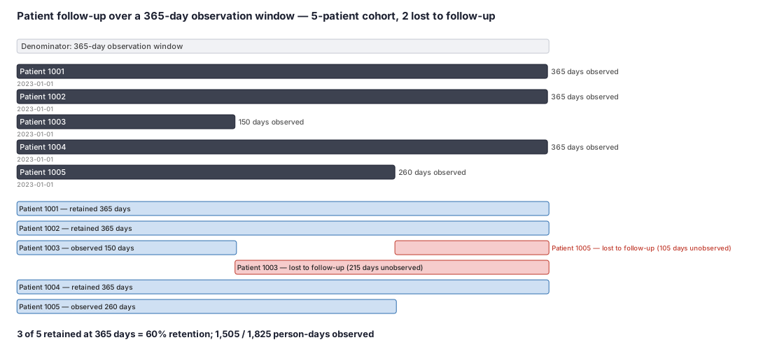
In the five-patient cohort, the audit log shows: patients 1001, 1002, and 1004 each contribute 365 person-days; patient 1003 is censored at day 150; patient 1005 at day 260. Total observed person-days = 1,505 of 1,825 possible (82.5% of potential follow-up); 365-day retention = 3/5 = 60%.

(1) Formal interpretation. The 60% retention rate signals that 40% of the cohort was lost before the intended 365-day endpoint. Whether this loss is informative depends on the reason for censoring relative to the outcome mechanism. If patients 1003 and 1005 disenrolled because of worsening disease — a process correlated with the event being counted — then standard administrative censoring produces a biased event rate (informative censoring). The 82.5% person-time capture is a secondary measure: high person-time percentage can coexist with heavy early-dropout bias if those lost early were the highest-risk patients in the cohort.

(2) Practical interpretation. A 60% retention rate at 12 months is a threshold most regulatory reviewers will flag for mandatory sensitivity analysis. The directional question is whether retained patients are systematically healthier or sicker than those lost. If the drug arm has higher dropout — for example, patients stopping due to adverse events — the surviving arm appears artificially healthier, and IPCW or a competing-risk model is required before the event rate can be interpreted as unbiased. Always stratify the attrition diagnostic by treatment arm to detect differential loss.

Worked example

Scenario

A health-plan database study enrolls 5 adults with a new diabetes diagnosis on January 1, 2023. The research team wants to track each patient for 365 days to count hospitalizations. Patients are observable as long as they remain enrolled in the health plan. Two patients disenroll before 365 days (they are lost to follow-up), and the team wants to summarize how much follow-up time they collected and what fraction of the original cohort remained at the end.

Dataset

Study roster: each row is one patient. 'days_observed' is person-time elapsed from January 1, 2023. Patients 1003 and 1005 disenrolled before the 365-day window closed.

Steps

• Each patient starts on January 1, 2023. The 365-day window closes January 1, 2024. Days observed = days of person-time elapsed from the start date (so a patient who exits on May 31 has contributed 150 days, because January 1 + 150 days = May 31).

• Patient 1001: still enrolled on January 1, 2024 — 365 days observed. Retained.

• Patient 1002: still enrolled on January 1, 2024 — 365 days observed. Retained.

• Patient 1003: disenrolled on May 31, 2023 (150 days after January 1). Their follow-up bar ends at day 150. The remaining 215 days of the window (365 − 150 = 215) are unobserved. Lost to follow-up.

• Patient 1004: still enrolled on January 1, 2024 — 365 days observed. Retained.

• Patient 1005: disenrolled on September 18, 2023 (260 days after January 1). Their follow-up bar ends at day 260. The remaining 105 days of the window (365 − 260 = 105) are unobserved. Lost to follow-up.

• Total person-days collected: 365 + 365 + 150 + 365 + 260 = 1,505 days out of a maximum possible 5 × 365 = 1,825 days.

• Patients retained at 365 days: patients 1001, 1002, and 1004 — 3 of the original 5.

• Retention rate: 3 ÷ 5 = 0.60, or 60%.

• Important caveat: if patients 1003 and 1005 disenrolled because they were hospitalized and lost insurance coverage — meaning sicker patients left first — then the 3 remaining patients are healthier on average than the full original cohort. Counting hospitalizations only among the survivors would undercount events. That is informative censoring introducing bias.

Result

Label

3 of 5 retained at 12 months = 60% retention; 1,505 of 1,825 possible person-days observed

Value

0.6

Timeline Spec

Title

Patient follow-up over a 365-day observation window — 5-patient cohort, 2 lost to follow-up

Window

Start

2023-01-01

End

2024-01-01

Label

Denominator: 365-day observation window

Events

• Label

  Patient 1001

  Start

  2023-01-01

  Length Days

  365

  Quantity

  365 days observed

• Label

  Patient 1002

  Start

  2023-01-01

  Length Days

  365

  Quantity

  365 days observed

• Label

  Patient 1003

  Start

  2023-01-01

  Length Days

  150

  Quantity

  150 days observed

• Label

  Patient 1004

  Start

  2023-01-01

  Length Days

  365

  Quantity

  365 days observed

• Label

  Patient 1005

  Start

  2023-01-01

  Length Days

  260

  Quantity

  260 days observed

Spans

• Kind

  followup

  Start

  2023-01-01

  End

  2024-01-01

  Label

  Patient 1001 — retained 365 days

  Row

  Patient 1001

• Kind

  followup

  Start

  2023-01-01

  End

  2024-01-01

  Label

  Patient 1002 — retained 365 days

  Row

  Patient 1002

• Kind

  followup

  Start

  2023-01-01

  End

  2023-05-31

  Label

  Patient 1003 — observed 150 days

  Row

  Patient 1003

• Kind

  gap

  Start

  2023-05-31

  End

  2024-01-01

  Label

  Patient 1003 — lost to follow-up (215 days unobserved)

  Row

  Patient 1003

• Kind

  followup

  Start

  2023-01-01

  End

  2024-01-01

  Label

  Patient 1004 — retained 365 days

  Row

  Patient 1004

• Kind

  followup

  Start

  2023-01-01

  End

  2023-09-18

  Label

  Patient 1005 — observed 260 days

  Row

  Patient 1005

• Kind

  gap

  Start

  2023-09-18

  End

  2024-01-01

  Label

  Patient 1005 — lost to follow-up (105 days unobserved)

  Row

  Patient 1005

Result

Label

3 of 5 retained at 365 days = 60% retention; 1,505 / 1,825 person-days observed

Value

0.6

Note

Patients 1003 and 1005 left at different points, so the at-risk cohort shrank over time — 5 patients at day 0, 4 after day 150, and 3 after day 260. If the patients who left were sicker than average (informative censoring), any outcome rate estimated from the 3 survivors will be too low.

Caption

Timeline showing 5 patients followed from January 1, 2023. Solid bars = days observed (follow-up); hatched bars = unobserved window after disenrollment. Patients 1003 and 1005 dropped out at days 150 and 260, respectively. Three of five patients (60%) remained observable through the full 365-day window.

Alt Text

Horizontal bar chart with one row per patient. Patients 1001, 1002, and 1004 each have a solid bar spanning the full 365-day window. Patient 1003 has a solid bar for the first 150 days and a hatched bar for the remaining 215 days. Patient 1005 has a solid bar for the first 260 days and a hatched bar for the remaining 105 days. A summary line at the bottom reads: 3 of 5 retained at 12 months = 60% retention.

Runnable example

import numpy as np
import pandas as pd
import statsmodels.formula.api as smf
from lifelines import KaplanMeierFitter

# ---- (1) Retention by arm: KM on the CENSORING distribution (event = loss to follow-up) ----
# A steep, arm-differential censoring curve is the signal that loss is informative.
cens = person.copy()
cens["lost"] = cens["exit_reason"].isin(["disenroll"]).astype(int)   # death handled as competing event, not loss
cens["fu_days"] = (cens["exit_date"] - cens["index_date"]).dt.days
kmf = KaplanMeierFitter()
for a, g in cens.groupby("arm"):
    kmf.fit(g["fu_days"], event_observed=g["lost"], label=f"arm {a}")
    print(a, "retention at 180d:", float(kmf.predict(180)))   # 1 - cumulative loss

# ---- (2) Stabilized IPCW via discrete-time pooled logistic for staying observable ----
# Numerator depends on arm only (baseline); denominator adds time-varying predictors of dropout.
num = smf.logit("observed_next ~ C(arm_t) + t + I(t**2)", data=panel).fit(disp=0)
den = smf.logit(
    "observed_next ~ C(arm_t) + t + I(t**2) + comorbidity + prior_hcru "
    "+ adherence + C(age_band) + recent_hosp",
    data=panel,
).fit(disp=0)

panel = panel.sort_values(["person_id", "t"]).copy()
panel["num_t"] = num.predict(panel).values   # P(stay observable | baseline)
panel["den_t"] = den.predict(panel).values   # P(stay observable | full history)
# Cumulative product within person = probability of remaining UNCENSORED through interval t.
panel["cum_num"] = panel.groupby("person_id")["num_t"].cumprod()
panel["cum_den"] = panel.groupby("person_id")["den_t"].cumprod()
panel["ipcw"] = panel["cum_num"] / panel["cum_den"]

# Truncate extreme weights at the 1st/99th percentile and report stability.
lo, hi = panel["ipcw"].quantile([0.01, 0.99])
panel["ipcw_trunc"] = panel["ipcw"].clip(lo, hi)
print("IPCW mean (should be ~1):", round(panel["ipcw_trunc"].mean(), 3),
      "max:", round(panel["ipcw_trunc"].max(), 2))
# Downstream: multiply ipcw_trunc by IPTW and pass as weights to a (pooled-logistic or Cox) outcome model.

library(dplyr)
library(survival)
library(cmprsk)

## ---- Stabilized IPCW from a discrete-time pooled logistic for staying observable ----
num <- glm(observed_next ~ factor(arm_t) + t + I(t^2),
           family = binomial, data = panel)
den <- glm(observed_next ~ factor(arm_t) + t + I(t^2) + comorbidity + prior_hcru +
             adherence + factor(age_band) + recent_hosp,
           family = binomial, data = panel)

panel <- panel %>%
  arrange(person_id, t) %>%
  mutate(p_num = predict(num, type = "response"),
         p_den = predict(den, type = "response")) %>%
  group_by(person_id) %>%
  mutate(ipcw = cumprod(p_num) / cumprod(p_den)) %>%
  ungroup()
qs <- quantile(panel$ipcw, c(0.01, 0.99))
panel$ipcw_trunc <- pmin(pmax(panel$ipcw, qs[1]), qs[2])   # weight truncation

## ---- IPCW-weighted Cox (per-protocol / no-informative-censoring estimand) ----
## Attach the last-interval weight to each person's survival record, then fit weighted Cox.
w <- panel %>% group_by(person_id) %>% summarise(w = dplyr::last(ipcw_trunc), .groups = "drop")
surv_w <- left_join(surv, w, by = "person_id")
fit_ipcw <- coxph(Surv(fu_time, status == 1) ~ arm, data = surv_w,
                  weights = w, robust = TRUE)   # robust SE required with weights
print(summary(fit_ipcw)$coefficients)

## ---- Competing risks: death (status==2) is a COMPETING EVENT, not censoring ----
## Cause-specific hazard (etiologic): standard Cox, censor at death.
fit_cs <- coxph(Surv(fu_time, status == 1) ~ arm, data = surv)
## Subdistribution hazard / cumulative incidence (absolute risk): Fine-Gray.
fg <- crr(ftime = surv$fu_time, fstatus = surv$status,
          cov1 = model.matrix(~ arm, surv)[, -1, drop = FALSE],
          failcode = 1, cencode = 0)   # failcode=1 event of interest, 2 treated as competing
print(summary(fg))