Retrospective Cohort Study Design

In plain language

A retrospective cohort study answers a cause-and-effect question (does taking drug A change a patient's risk of outcome B?) using health records that were already collected for other reasons, like insurance billing or routine care. The analyst picks a 'day zero' for each patient that sits in the past, splits people into groups by what treatment they were on at that moment, and then reads forward through the already-written record to see who had the outcome. The follow-up still runs forward in time, exactly like a study that enrolls patients and waits; the only difference is that everything has already happened by the time the researcher sits down. Its big payoff is speed and size, but it can only ever measure things the original record happened to capture.

A retrospective cohort (also historical or non-concurrent cohort) follows the same exposure-to-outcome logic as a prospective cohort, but does so inside data that already exist. The investigator identifies a cohort by exposure status at a past time-zero (index), then "follows" each person forward through the recorded data — claims, electronic health records (EHR), registries, or linked sources — to observe outcomes, censoring, resource use, or other endpoints that have, in calendar time, already happened. The defining feature is temporality of data capture, not the direction of inference: like any cohort, it moves exposure → outcome; unlike a prospective cohort, the data were collected before the research question was posed and for reasons other than the study (billing, care delivery, surveillance).

Core conceptual distinction — design vs estimand vs data

Three things must be held apart and pre-specified. (1) The design fixes time-zero, eligibility, the exposure contrast, and the censoring rules. (2) The estimand — the causal contrast (e.g., a per-protocol vs intention-to-treat-analogue hazard ratio, cumulative incidence, or rate difference) and the target population — dictates the model, not the reverse. A retrospective cohort can support a cause-specific hazard, a subdistribution effect under competing risks, restricted mean survival time, or a rate ratio; the design does not choose for you. (3) The data constrain which estimands are even identifiable. The modern, defensible way to specify all three at once is target-trial emulation: write down the protocol of the randomized trial you wish you could run (eligibility, treatment strategies, assignment, time-zero, outcome, causal contrast, analysis), then build the retrospective cohort to emulate it. Retrospective cohorts that are not anchored to an explicit time-zero and a clear estimand are where immortal time, prevalent-user bias, and post-baseline adjustment silently enter.

Pros, cons, and trade-offs

- vs prospective cohort: The retrospective cohort uses data that already exist, so it is fast, large, inexpensive at the margin, and can deliver long follow-up the day the study starts — decisive when the outcome is rare or the latency is long, or when prospective enrollment would be unethical or impractical. Cost: you are limited to what was recorded; no biospecimens, no protocolized PROs, no adjudicated endpoints at fixed visits unless you add linkage or a hybrid arm. Prefer retrospective for comparative safety/effectiveness, drug-utilization, and HCRU questions where the constructs are codeable; prefer prospective when the exposure or outcome cannot be reconstructed from routine data with acceptable misclassification. - vs nested case-control / case-cohort within the same source: The full retrospective cohort retains person-time for every member, supports time-varying exposure and absolute-risk estimands, and is reusable for multiple outcomes. Cost: it is more computationally and data-management intensive than sampling controls. Prefer the full cohort when you need rates, cumulative incidence, or several endpoints; prefer nested sampling when an expensive covariate (chart review, biomarker) must be collected on a subset. - vs self-controlled designs (SCCS, case-crossover): Self-controlled designs eliminate all time-fixed confounding by using the person as their own control, which a between-person retrospective cohort cannot. Cost: they require a transient exposure and an acute outcome and cannot estimate effects of stable exposures. Prefer self-controlled for acute-on-transient questions (e.g., vaccine-fever); prefer the cohort for chronic therapies and absolute risk. - vs prevalent-user / cross-sectional analyses of the same data: A new-user retrospective cohort aligns time-zero at initiation and so avoids depletion of susceptibles and adjustment for post-initiation variables. Cost: smaller N and a population skewed toward initiators. This is a variant choice within the retrospective cohort, not a different data source.

When to use

Comparative effectiveness or safety of treatments codeable in routine data; incidence, prevalence, and natural-history questions; HCRU and cost endpoints; long-latency or rare outcomes where prospective follow-up is infeasible; and as the data-construction backbone of any target-trial emulation. The design is appropriate whenever a defensible time-zero, an observable exposure contrast, and validated outcome and covariate definitions can be built from the source.

When NOT to use — and when it is actively misleading or dangerous

- No clean time-zero exists. If you start follow-up at a point everyone in one arm has already survived to (e.g., follow-up from a procedure date but classifying exposure by a prescription filled later), you manufacture immortal time that spuriously favors the exposed. If you cannot place a single, arm-symmetric time-zero, do not run the cohort as specified — restructure or use a self-controlled design. - Exposure or outcome cannot be reconstructed. Over-the-counter drugs, inpatient-administered agents invisible in pharmacy claims, samples, and outcomes with no validated algorithm produce differential misclassification that no adjustment fixes. - Prevalent-user contrast with depletion of susceptibles. Comparing current users to non-users on routine data embeds survivor bias and adjustment for mediators; a naive prevalent-user cohort here is worse than no study. - Person-time is unobservable or differentially missing. In claims, Medicare Advantage (MA) enrollees generate no fee-for-service (FFS) claims, so their exposures and outcomes are invisible; counting MA person-time as "unexposed and event-free" biases rates. Likewise, EHR follow-up ends silently when a patient leaves the system. - Competing risks ignored in an elderly or sick cohort. When death competes with the outcome and competing-event rates differ by exposure (common in older claims populations), a naive cause-specific Kaplan-Meier over-states cumulative incidence; the estimand (cause-specific vs subdistribution) must be chosen deliberately.

Data-source operational depth

- Claims (FFS or commercial): The substrate is eligibility, medical, and pharmacy files. Establish observable person-time from enrollment spans, and require continuous enrollment (medical + pharmacy) across the full lookback so that "no prior event" is genuine absence, not unobserved care. Exposure comes from pharmacy claims (`ndc`, `fill_date`, `days_supply`) and procedures (CPT/HCPCS, ICD-10-PCS); diagnoses (ICD-10-CM) serve eligibility, covariates, and validated outcome algorithms. Failure modes and workarounds: (a) MA-only person-time lacks FFS claims — restrict to enrollees with the relevant benefit (Parts A/B/D, or commercial medical+pharmacy) and exclude MA-only spans rather than treating them as event-free; (b) adjudication/claims lag truncates recent person-time — apply a data-cutoff buffer or restrict to fully run-out claims; (c) 90-day mail-order and free samples distort `days_supply` and washout — model supply windows explicitly; (d) death is often unobserved in commercial claims — link to a death index or treat disenrollment as potentially informative censoring. - EHR: Richer baseline (labs, vitals, severity, notes via NLP) and some outcomes, but visit-driven, irregular observation: a patient who stops visiting is differentially lost, not event-free. Define observation windows and a loss-to-follow-up rule (e.g., no encounter > N months) explicitly. Exposure is the order/administration, not the dispensing — link to pharmacy fills to confirm the patient actually started. Hybridize with claims for complete pharmacy and HCRU capture. - Registry: Strong, validated phenotypes and clinical endpoints (cancer stage, adjudicated events) but typically incomplete longitudinal exposure; link to claims for the full fill history and to a death index for censoring. Registry inclusion criteria bound generalizability. - Linked claims–EHR–vital records: Maximizes exposure completeness, baseline severity, and mortality, but linkage selects only the linkable subset and creates order/fill/service date discrepancies that must be reconciled before time-zero assignment; propagate linkage uncertainty into sensitivity analyses.

Worked claims example

Question: among adults with type 2 diabetes initiating a second-generation sulfonylurea, what is the 2-year cumulative incidence of hospitalized heart failure, in a commercial + Medicare FFS database? (1) Source population and eligibility: age ≥ 18, ≥ 2 outpatient or 1 inpatient diabetes diagnosis (ICD-10-CM E11.x), and 365 days of continuous medical + pharmacy (or A/B/D) enrollment before the first qualifying fill, with all MA-only person-time excluded. (2) Time-zero / index: the date of the first sulfonylurea fill (`ndc` on `fill_date`) after a clean 365-day washout with no prior sulfonylurea dispensing — this makes the cohort incident users and fixes a single, well-defined start of follow-up. (3) Exposure assignment: defined at index from the dispensed `ndc`; an as-treated variant would stitch `days_supply` into episodes with a grace period and censor at discontinuation. (4) Baseline covariates: measured only in the 365-day pre-index window (comorbidities, prior insulin, baseline HCRU, comorbidity index) — never using any post-index information, to avoid conditioning on mediators. (5) Follow-up and outcome: from index to the first hospitalized HF event (a validated inpatient ICD-10-CM algorithm), applied identically across the cohort. (6) Censoring: at disenrollment (from eligibility spans), death (linked index), end of data, or 2 years, whichever comes first — and, because death competes with HF in this older population, report the subdistribution cumulative incidence (Fine-Gray / Aalen-Johansen) rather than a naive 1−KM. (7) Sensitivity: vary washout length (180 vs 365 days), redefine the grace period for the as-treated analysis, and add a negative-control outcome to probe residual confounding.

Worked example

Scenario

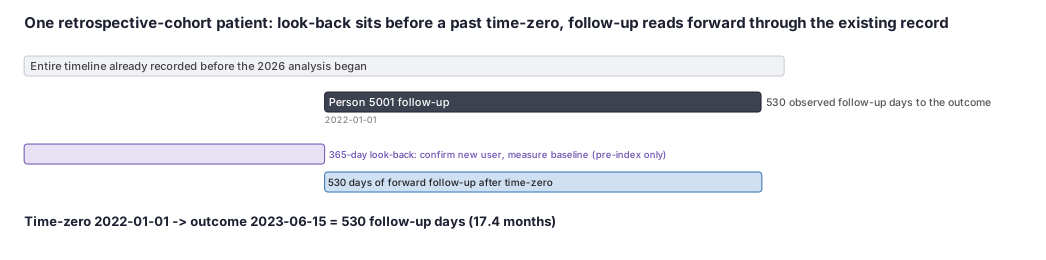
It is 2026 and we want to know whether adults who start a new diabetes pill go on to be hospitalized for heart failure. Instead of enrolling patients and waiting two years, we open an insurance claims database that already covers 2021 through early 2024. We follow one patient, person 5001, who first filled the new pill on 2022-01-01. Everything in this story already happened years ago; our job is just to read the record in the right order, looking back before that fill to confirm she is a new user, then looking forward to see if and when the outcome occurred.

Dataset

The kind of rows an analyst actually sees: one enrollment span telling us when the insurer could observe her, plus the dated events (a prior fill check, her first qualifying fill, and a later hospitalization).

Steps

• Set time-zero (day zero) to her first qualifying fill on 2022-01-01; this is the day she joins the new-user group, and it sits squarely in the past.

• Look BACK across the 365 days before time-zero (2021-01-01 to 2021-12-31) and confirm she had continuous coverage and no earlier fill of this drug class, so she truly is a brand-new user and we can measure her starting health from that window only.

• Look FORWARD from time-zero through the already-written record, watching for the outcome; she is hospitalized for heart failure on 2023-06-15.

• Count the follow-up time from day zero to the event: 2022-01-01 to 2023-06-15 is 530 days, about 17.4 months.

• If no event had appeared, we would have followed her until coverage ended or until a fixed 2-year (730-day) cap, then censored her there rather than assume she stayed event-free.

Result

Follow-up from time-zero (2022-01-01) to the heart-failure hospitalization (2023-06-15) = 530 days = 17.4 months. This single event would later be pooled with every other patient's person-time to estimate a rate; the design's whole job was to place day zero correctly and read look-back before it and follow-up after it.

Timeline Spec

Title

One retrospective-cohort patient: look-back sits before a past time-zero, follow-up reads forward through the existing record

Window

Start

2021-01-01

End

2024-01-01

Label

Entire timeline already recorded before the 2026 analysis began

Events

• Label

  Person 5001 follow-up

  Start

  2022-01-01

  Length Days

  530

  Quantity

  530 observed follow-up days to the outcome

Spans

• Kind

  washout

  Start

  2021-01-01

  End

  2021-12-31

  Label

  365-day look-back: confirm new user, measure baseline (pre-index only)

• Kind

  followup

  Start

  2022-01-01

  End

  2023-06-15

  Label

  530 days of forward follow-up after time-zero

Result

Label

Time-zero 2022-01-01 -> outcome 2023-06-15 = 530 follow-up days (17.4 months)

Value

530

Caption

Time-zero (2022-01-01) sits in the past. To its left is the 365-day look-back the analyst reads to confirm a new user and capture baseline health; to its right is forward follow-up through the already-recorded data, ending at the heart-failure event on day 530. The follow-up direction is forward, identical to a prospective study; only the recording happened earlier.

Alt Text

Horizontal timeline from 2021 to early 2024. A shaded 365-day look-back block runs from 2021-01-01 to 2021-12-31, then a time-zero marker at 2022-01-01, then a longer forward follow-up block of 530 days ending at an outcome marker on 2023-06-15. A note states the whole timeline was already recorded before the 2026 analysis.

Runnable example

import pandas as pd

WASHOUT_DAYS = 365   # clean lookback that defines an incident (new) user
MAX_FOLLOWUP = 730   # 2-year administrative cap

def build_retro_cohort(events: pd.DataFrame, enroll: pd.DataFrame) -> pd.DataFrame:
    events = events.sort_values(["person_id", "event_date"])

    # Time-zero = first qualifying event per person.
    idx = (events.groupby("person_id", as_index=False)
                 .first()
                 .rename(columns={"event_date": "index_date"}))

    # New-user check: no qualifying event in the WASHOUT_DAYS before index.
    prior = events.merge(idx[["person_id", "index_date"]], on="person_id")
    had_prior = prior[(prior["event_date"] < prior["index_date"]) &
                      (prior["event_date"] >= prior["index_date"] - pd.Timedelta(days=WASHOUT_DAYS))]
    idx = idx[~idx["person_id"].isin(had_prior["person_id"])].copy()

    # Continuous, FFS-OBSERVABLE enrollment spanning the full washout through index (no MA-only spans).
    e = enroll.merge(idx[["person_id", "index_date"]], on="person_id")
    covers_baseline = ((e["enroll_start"] <= e["index_date"] - pd.Timedelta(days=WASHOUT_DAYS)) &
                       (e["enroll_end"]   >= e["index_date"]) &
                       (~e["ma_only"]))
    eligible = e.loc[covers_baseline, "person_id"].unique()
    cohort = idx[idx["person_id"].isin(eligible)].copy()

    # Observable follow-up END = first of: end of the FFS span covering index, or the admin cap.
    post = enroll[(~enroll["ma_only"])].merge(cohort[["person_id", "index_date"]], on="person_id")
    post = post[(post["enroll_start"] <= post["index_date"]) & (post["enroll_end"] >= post["index_date"])]
    span_end = post.groupby("person_id")["enroll_end"].max()
    cohort = cohort.join(span_end.rename("ffs_end"), on="person_id")

    cohort["baseline_start"] = cohort["index_date"] - pd.Timedelta(days=WASHOUT_DAYS)  # covariate window
    admin_cap = cohort["index_date"] + pd.Timedelta(days=MAX_FOLLOWUP)
    cohort["censor_date"] = cohort[["ffs_end"]].assign(cap=admin_cap).min(axis=1)      # +death/outcome downstream
    return cohort[["person_id", "index_date", "baseline_start", "censor_date"]]

library(data.table)
WASHOUT_DAYS <- 365L
MAX_FOLLOWUP <- 730L

build_retro_cohort <- function(events, enroll) {
  setDT(events); setDT(enroll)
  setorder(events, person_id, event_date)

  # Time-zero = first qualifying event per person.
  idx <- events[, .(index_date = event_date[1L]), by = person_id]

  # New-user: drop anyone with a qualifying event in the washout window before index.
  ev <- merge(events, idx, by = "person_id")
  prior_ids <- unique(ev[event_date < index_date &
                         event_date >= index_date - WASHOUT_DAYS, person_id])
  idx <- idx[!person_id %chin% prior_ids]

  # Continuous, FFS-observable enrollment across the full washout through index.
  e <- merge(enroll, idx, by = "person_id")
  ok <- e[enroll_start <= index_date - WASHOUT_DAYS &
          enroll_end   >= index_date & !ma_only, unique(person_id)]
  cohort <- idx[person_id %chin% ok]

  # Observable follow-up end = end of FFS span covering index, capped at MAX_FOLLOWUP.
  post <- merge(enroll[ma_only == FALSE], cohort, by = "person_id")
  post <- post[enroll_start <= index_date & enroll_end >= index_date]
  ffs  <- post[, .(ffs_end = max(enroll_end)), by = person_id]
  cohort <- merge(cohort, ffs, by = "person_id", all.x = TRUE)

  cohort[, baseline_start := index_date - WASHOUT_DAYS]
  cohort[, censor_date := pmin(ffs_end, index_date + MAX_FOLLOWUP)]  # +death/outcome downstream
  cohort[, .(person_id, index_date, baseline_start, censor_date)]
}