Prospective Cohort Study

In plain language

A prospective cohort study starts with a group of people sorted by whether they did or did not get a treatment, marks that starting moment as everyone's day zero, and then watches them move forward in time to see who later develops the outcome you care about. Because you decide who's in which group before any outcomes happen, you get to measure things in the same order you want to reason about them: cause first, effect second. The payoff is that you can directly count how often the outcome happens (the actual risk), and you can track several different outcomes from the same starting group. The catch is that it's slow and wasteful when the outcome is very rare, since you have to watch a lot of people to catch a few events.

A prospective cohort study classifies people by exposure at a defined time origin (time zero) and then follows them forward to observe who develops the outcome. The defining feature is temporal: exposure status and baseline covariates are fixed and recorded before any outcome is known, so the direction of measurement matches the direction of inference. This is what distinguishes it from a retrospective cohort (where both exposure and outcome have already occurred when the investigator looks) and from a case-control study (which samples on the outcome and looks backward at exposure). In real-world data the "prospective" label is often about analytic posture rather than wall-clock timing: a study built in an administrative database is technically conducted on already-accrued records, but it is designed and analyzed prospectively when the protocol fixes eligibility, time zero, exposure, and covariate windows a priori and follows each person forward from time zero — the structure Hernán and Robins formalize as target-trial emulation.

Core conceptual / estimand distinction

A cohort is a sampling-and-follow-up frame, not an estimator. The design fixes who is in the risk set, when their clock starts, and what counts as person-time at risk; the estimand (cumulative incidence, incidence rate, hazard ratio, risk difference, restricted mean survival time) and the confounding-control strategy (restriction, matching, propensity scores, g-methods) are layered on top. The cohort frame delivers two things a case-control design cannot: it lets you estimate absolute risks and rates directly (numerator events over a denominator of person-time you actually counted), and it lets you study multiple outcomes from a single exposure definition. Getting the frame right — one unambiguous time zero per person, exposure assigned at time zero, covariates measured before time zero, follow-up that begins at time zero — is the work; nearly every notorious cohort bias is a violation of one of those four rules.

Pros, cons, and trade-offs

- vs case-control: A cohort yields incidence and absolute risk, handles many outcomes at once, and avoids the recall and selection biases that plague exposure ascertainment after the outcome is known. Cost: it is inefficient for rare outcomes (you must follow large denominators for few events) and for outcomes with long induction periods. Prefer a cohort when the exposure is rare or when absolute risk / multiple outcomes matter; prefer nested case-control or case-cohort sampling within the cohort when an expensive covariate (biomarker, chart abstraction, adjudication) must be collected and the outcome is rare. - vs retrospective cohort: Prospective measurement (or prospective design in RWD) lets you specify exposure and confounders before knowing outcomes, which protects against data-driven definition tweaking and against conditioning on post-baseline variables. Cost: in primary-data collection it is slower and more expensive; in RWD the trade is that you are limited to variables the data captured, captured before time zero. - vs cross-sectional: A cohort establishes temporality (exposure precedes outcome), the single most important ingredient for causal interpretation, which a cross-sectional snapshot cannot. Cost: follow-up infrastructure, loss to follow-up, and competing risks. - vs RCT: A cohort can study harms, long-term outcomes, rare exposures, and populations excluded from trials, at real-world scale and cost. Cost: treatment assignment is not randomized, so confounding (especially confounding by indication) is the central threat and must be addressed by design (active comparator, new-user restriction) and analysis (PS methods, negative controls), not assumed away.

When to use

Estimating incidence or absolute risk; comparing outcomes across exposure groups when the exposure is reasonably common; studying multiple outcomes of one exposure; long-term safety and effectiveness questions; any setting where you can define a clean time zero and measure confounders before it. In pharmacoepidemiology the prospective cohort is the default frame, almost always implemented as a new-user (incident-user) cohort with an active comparator so that follow-up starts at initiation for everyone and the two arms cleared the same clinical threshold to be treated.

When NOT to use — and when it is actively misleading or dangerous

- Very rare outcomes with expensive covariates. Following a huge cohort to capture a handful of events wastes measurement resources; a nested case-control or case-cohort design recovers nearly all the efficiency at a fraction of the cost. Forcing a full cohort here is not wrong, but it is the wrong tool. - Ill-defined or person-varying time zero. If time zero is set at a point that itself depends on future events (e.g., starting follow-up at diagnosis but classifying exposure by a treatment received later), you manufacture immortal time bias: exposed person-time before the drug is dispensed is guaranteed event-free and spuriously favors the exposed. This is the single most common fatal error in RWD cohorts and is actively misleading — it can invert the sign of an effect. - Prevalent-user (ever-exposed) cohorts. Starting follow-up among current users mixes people at different points in their treatment trajectory, induces depletion of susceptibles (survivors tolerate the drug and look healthier), and forces adjustment for variables on the causal pathway. Use a new-user cohort unless initiation is too rare, in which case consider the prevalent-new-user (Suissa) extension. - Differential loss to follow-up by exposure. If the exposed and unexposed are censored for outcome-related reasons at different rates (informative censoring), naive estimates are biased; this demands explicit observation windows and, often, inverse-probability-of-censoring weighting. - No way to control confounding by indication. A cohort comparing treated vs untreated for a condition that itself predicts the outcome, with no active comparator and no measured confounders, produces a confounded contrast that looks quantitative but is not interpretable as causal.

Data-source operational depth

- Claims (FFS or commercial): The natural substrate for incident-user cohorts. Exposure = the pharmacy claim (NDC + `fill_date` + `days_supply`); diagnoses come from medical claims (ICD-10-CM on professional/facility lines). Require continuous medical + pharmacy enrollment across the whole baseline/washout window so that "no prior fill" is a real observation, not unobserved person-time. Failure modes: (1) Medicare Advantage / capitated person-time lacks fee-for-service claims — utilization and fills are invisible, so absence of an event or a prior fill is missingness; restrict to enrollees with Parts A/B/D (or a commercial medical+pharmacy benefit) and drop MA-only spans. (2) Differential competing risks by exposure in elderly claims — death is a competing event that is often unobserved unless a death index or Part A inpatient-discharge-status is linked; if one arm is older/sicker, ignoring the competing risk overstates the cumulative incidence of the event of interest (use Fine-Gray or report cause-specific and cumulative-incidence estimates). (3) Immortal time in procedure/treatment studies — defining the exposed group by receipt of a procedure but starting the clock at an earlier landmark builds guaranteed survival into the exposed; align time zero to the procedure or use a landmark/time-varying treatment. - EHR: Time zero is the order or administration, not a dispensing; problem lists, labs, and notes sharpen indication and baseline severity (an advantage over claims), but visit-driven capture means a patient who leaves the system disappears — define observation windows explicitly and treat loss to follow-up as potentially informative. Linkage to pharmacy fills is preferred to confirm the patient actually started. - Registry: Strongest for indication, disease severity, and adjudicated/validated outcomes (e.g., cancer stage, cause of death); typically weak for complete medication exposure and for non-registry comorbidity. Link to claims for the full fill history and to a death index to firm up censoring. - Linked claims–EHR–vital records: The ideal substrate (EHR severity + claims completeness + reliable mortality), but linkage introduces selection (only the linkable subset) and date-discrepancy issues (order vs fill vs service date) that must be reconciled before time zero is assigned.

Worked claims example

Question: 2-year cumulative incidence of hospitalized GI bleed among adults initiating a non-selective NSAID, in a commercial + Medicare FFS database. (1) Eligibility: age ≥18 and ≥365 days of continuous medical + pharmacy enrollment before the first NSAID fill (FFS-observable, no MA-only spans). (2) Washout: no NSAID fill in the 365-day lookback — this makes the cohort incident users and removes prevalent-user bias. (3) Time zero: the date of that first qualifying fill (the `fill_date` of the index NDC). (4) Baseline covariates: measured only in the 365 days up to and including time zero (prior GI bleed, anticoagulant/antiplatelet use, age, utilization), so no covariate is on the causal pathway. (5) Follow-up and person-time: from time zero forward to the first inpatient claim with a primary GI-bleed diagnosis; censor at disenrollment, death (from a linked death index — a competing event, not an outcome), 2 years, or end of data. Do not count post-`days_supply` time as immortal "exposed" time — if this is an as-treated analysis, the on-treatment window is the stitched `days_supply` episodes plus a pre-specified grace period. (6) Estimand: report the cumulative incidence function treating death as a competing risk (not 1 − KM), plus the incidence rate per 1,000 person-years; compare exposure groups with an active comparator (e.g., a different analgesic class) and PS adjustment rather than against never-users.

Worked example

Scenario

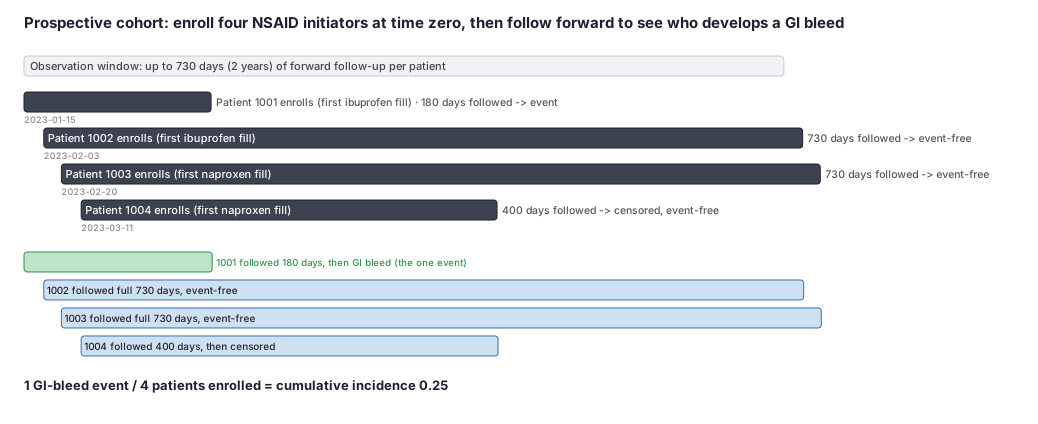
We want the 2-year (730-day) risk of a hospitalized GI bleed among adults who start taking an NSAID pain reliever. We have a tiny claims dataset of four patients, each with the pharmacy fill that marks their first NSAID. We set each person's day zero to that first fill, then follow every patient forward to see who is hospitalized for a GI bleed before two years are up. We then count the events and divide by the four people we started with.

Dataset

The raw rows an analyst would see: one starting fill per patient, plus what happened during forward follow-up.

Steps

• For each patient, day zero is their first NSAID fill_date, and the clock starts there and only moves forward.

• Patient 1001 is hospitalized for a GI bleed 180 days after starting, so they count as one event.

• Patients 1002 and 1003 are watched the full 730 days and never have the event.

• Patient 1004 leaves their insurance plan at day 400, so we stop watching them with no event recorded; they are censored but still part of the four people we started with.

• Count the events (1) and divide by the number of people who started (4).

Result

2-year cumulative incidence = 1 GI-bleed event / 4 patients enrolled at time zero = 0.25, or about 25%.

Timeline Spec

Title

Prospective cohort: enroll four NSAID initiators at time zero, then follow forward to see who develops a GI bleed

Window

Start

2023-01-15

End

2025-01-14

Label

Observation window: up to 730 days (2 years) of forward follow-up per patient

Events

• Label

  Patient 1001 enrolls (first ibuprofen fill)

  Start

  2023-01-15

  Length Days

  180

  Quantity

  180 days followed -> event

• Label

  Patient 1002 enrolls (first ibuprofen fill)

  Start

  2023-02-03

  Length Days

  730

  Quantity

  730 days followed -> event-free

• Label

  Patient 1003 enrolls (first naproxen fill)

  Start

  2023-02-20

  Length Days

  730

  Quantity

  730 days followed -> event-free

• Label

  Patient 1004 enrolls (first naproxen fill)

  Start

  2023-03-11

  Length Days

  400

  Quantity

  400 days followed -> censored, event-free

Spans

• Kind

  exposed

  Start

  2023-01-15

  End

  2023-07-14

  Label

  1001 followed 180 days, then GI bleed (the one event)

• Kind

  followup

  Start

  2023-02-03

  End

  2025-02-02

  Label

  1002 followed full 730 days, event-free

• Kind

  followup

  Start

  2023-02-20

  End

  2025-02-19

  Label

  1003 followed full 730 days, event-free

• Kind

  followup

  Start

  2023-03-11

  End

  2024-04-14

  Label

  1004 followed 400 days, then censored

Result

Label

1 GI-bleed event / 4 patients enrolled = cumulative incidence 0.25

Value

0.25

Runnable example

import pandas as pd

WASHOUT_DAYS = 365   # drug-free + continuous-enrollment lookback that makes a user "incident"
STUDY_NDCS = {...}   # set of NDCs defining the exposure of interest

def build_prospective_cohort(rx: pd.DataFrame, enroll: pd.DataFrame) -> pd.DataFrame:
    rx = rx.sort_values(["person_id", "fill_date"])
    study = rx[rx["ndc"].isin(STUDY_NDCS)]

    # Candidate time zero = first fill of the study exposure for each person.
    idx = (study.groupby("person_id", as_index=False)
                .first()
                .rename(columns={"fill_date": "index_date"})[["person_id", "index_date"]])

    # New-user restriction: no study fill in the washout window strictly before time zero.
    prior = study.merge(idx, on="person_id")
    prior_in_washout = prior[(prior["fill_date"] < prior["index_date"]) &
                             (prior["fill_date"] >= prior["index_date"] - pd.Timedelta(days=WASHOUT_DAYS))]
    idx = idx[~idx["person_id"].isin(prior_in_washout["person_id"])].copy()

    # Continuous, FFS-observable enrollment spanning the full washout through time zero (no MA-only gaps).
    e = enroll.merge(idx, on="person_id")
    e["covers"] = ((e["enroll_start"] <= e["index_date"] - pd.Timedelta(days=WASHOUT_DAYS)) &
                   (e["enroll_end"]   >= e["index_date"]) &
                   (~e["ma_only"]))
    eligible = e.loc[e["covers"], "person_id"].unique()

    cohort = idx[idx["person_id"].isin(eligible)].copy()
    # Baseline covariate window: measure confounders strictly up to and including time zero (never after).
    cohort["baseline_start"] = cohort["index_date"] - pd.Timedelta(days=WASHOUT_DAYS)
    # Follow-up starts AT time zero -> no immortal time. Censoring (disenroll/death/end-of-data) added downstream.
    cohort["followup_start"] = cohort["index_date"]
    return cohort[["person_id", "index_date", "baseline_start", "followup_start"]]

library(data.table)
WASHOUT_DAYS <- 365L
STUDY_NDCS <- c(...)  # NDCs defining the exposure of interest

build_prospective_cohort <- function(rx, enroll) {
  setDT(rx); setDT(enroll)
  setorder(rx, person_id, fill_date)
  study <- rx[ndc %chin% STUDY_NDCS]

  # Candidate time zero = first study fill per person.
  idx <- study[, .(index_date = fill_date[1L]), by = person_id]

  # New-user restriction: drop anyone with a study fill in the washout window before time zero.
  study <- merge(study, idx, by = "person_id")
  prior_ids <- unique(study[fill_date < index_date &
                            fill_date >= index_date - WASHOUT_DAYS, person_id])
  idx <- idx[!person_id %chin% prior_ids]

  # Continuous, FFS-observable enrollment across the full washout through time zero (no MA-only spans).
  e <- merge(enroll, idx, by = "person_id")
  ok <- e[enroll_start <= index_date - WASHOUT_DAYS &
          enroll_end   >= index_date & !ma_only, unique(person_id)]

  cohort <- idx[person_id %chin% ok]
  cohort[, baseline_start := index_date - WASHOUT_DAYS]  # covariate window ends at time zero
  cohort[, followup_start := index_date]                 # follow-up begins at time zero -> no immortal time
  cohort[, .(person_id, index_date, baseline_start, followup_start)]
}