Medication Possession Ratio (MPR)

In plain language

The Medication Possession Ratio (MPR) measures how much medication a patient picked up from the pharmacy relative to how long they were supposed to be on it. You add up the total days' worth of pills dispensed across all prescription fills during the study period, then divide by the number of days in that period. Unlike the Proportion of Days Covered (PDC), which counts only the unique calendar days a patient had pills on hand (and therefore stays at or below 100%), MPR simply adds raw supply — so when a patient refills early and two fills overlap, those overlapping days get counted twice in the numerator, and the result can exceed 1.0 (or 100%). That "over 100%" signal is not a flaw to hide; it tells you the patient was stockpiling supply.

Medication Possession Ratio (MPR)

is the oldest and still one of the most common refill-based ("secondary") adherence measures derived from pharmacy dispensing records or claims. In its canonical (simple, uncapped) form, MPR = (sum of `days_supply` across fills in the interval) / (number of days in the interval). It estimates the proportion of the interval during which the patient possessed enough medication to take it as prescribed. Because the numerator sums supply without regard to whether two fills cover the same calendar day, an early refill or a 90-day mail-order fill stacked on a retail fill can push MPR above 1.0 — a value that has no coherent interpretation as "fraction of days covered."

Core conceptual distinction

— MPR and PDC answer almost the same question with one decisive difference in how they treat overlap. PDC (proportion of days covered) is a set-cardinality measure: it counts the number of unique calendar days in the interval on which the patient had any supply on hand, divided by interval days; overlapping supply is counted once, so PDC is bounded in [0, 1] and stockpiled days carry forward only as future coverage. MPR is a quantity measure: it sums total supply acquired, so overlap is double-counted and the ceiling is broken. The practical consequence is systematic: uncapped MPR ≥ PDC for the same patient and window, and the gap grows with early refilling and supply stockpiling. The right framing of the estimand therefore matters — if the research question is "what share of time was this patient covered?" PDC (or capped MPR) is the target; if it is "how much drug did this patient acquire relative to need?" (a supply/utilization or cost question), uncapped MPR is the natural quantity. Choosing MPR for an "adherent vs non-adherent" dichotomy and then capping ad hoc at 1.0 silently redefines the measure into a coarse PDC, and reproducibility demands the cap and overlap rules be pre-specified.

Pros, cons, and trade-offs

- vs PDC (pdc-proportion-of-days-covered): MPR is computationally trivial (one SUM, one division — no day-level set construction), preserves the magnitude of oversupply (useful for waste, cost, and supply-chain analyses), and maintains comparability with the large pre-2010 literature and some legacy HEDIS-era reporting. Cost: uncapped MPR overestimates coverage whenever fills overlap, produces uninterpretable >100% values, and is not the PQA/CMS-endorsed measure for the Medicare Part D Star Ratings adherence triple-weighted measures (diabetes, hypertension RAS-antagonists, statins) — those use PDC. Prefer PDC for almost all contemporary comparative-effectiveness, quality-measurement, and regulatory work; prefer MPR only for total-acquisition/cost questions or explicit historical replication. - vs capped MPR (MPR truncated at 1.0): Capping removes the absurd >100% values and makes MPR converge toward PDC, but it is not identical to PDC: capping is applied to the summed ratio after the fact, whereas PDC removes overlap at the day level, so the two can still disagree when fills overlap heavily within the window (capped MPR caps the whole interval at 1.0 but does not reallocate stockpiled days to later gaps the way carry-over PDC does). Prefer the shift-forward (date-adjusted) variant if you want overlap to push later coverage outward rather than be discarded. - vs persistence (persistence-time-to-discontinuation): MPR measures intensity of coverage within a fixed denominator window and says nothing about when therapy stopped; persistence measures duration until a permissible-gap is exceeded. A patient can be highly persistent yet have low MPR (chronically under-refilling) or non-persistent yet high MPR over the period they were on therapy. Report both for a complete adherence picture; never substitute one for the other.

When to use

— use MPR when (1) the question is genuinely about total medication acquisition or supply relative to need (pharmacy cost, oversupply/waste, dose-adjustment surveillance), (2) you must replicate or pool with older studies that reported MPR, or (3) you need a fast first-pass adherence screen on a single-drug, single-window cohort with little expected overlap. In all three cases pre-specify the window, the overlap rule, and whether you cap at 1.0.

When NOT to use — and when it is actively misleading or dangerous

- As the adherence metric for quality reporting or a regulated effectiveness endpoint. PQA-defined PDC is the standard for CMS Star Ratings; submitting uncapped MPR (or silently capping it) misrepresents performance and is not defensible to FDA/EMA/HTA reviewers who expect PDC for "proportion covered." - When supply overlap is structural and differential. In therapies with 90-day mail-order, free manufacturer samples, dose titration, or PRN use, uncapped MPR inflates, and if overlap differs by exposure arm (e.g., one drug favored for mail-order), the bias is differential and can manufacture or mask an adherence-outcome association. This is the dangerous case: the measure is not just noisy, it is confounded. - As an exposure that is itself on the causal pathway. Conditioning on or matching on post-baseline MPR (a time-updated consequence of being on and tolerating the drug) induces healthy-adherer bias and collider/mediator bias — adherent patients are healthier in ways unmeasured in claims. Use MPR as an outcome or pre-specified time-varying exposure with appropriate g-methods, not as a baseline confounder. - As a switching/combination summary across a drug class without a class-level day map: summing `days_supply` across two interchangeable agents double-counts overlap days and breaks the measure; build a class-level coverage map first.

Data-source operational depth

- Administrative claims (FFS): The native substrate. MPR needs only `person_id`, `fill_date` (service date), and `days_supply` (plus NDC to define the cohort). Require continuous pharmacy + medical enrollment spanning the full observation window so that a missing fill is a true non-fill, not unobserved care. Failure modes: `days_supply` is miscoded for insulin, inhalers, topicals, and titrated drugs (canister/vial counts, not days); the last fill's supply extends past the window end and inflates a fixed-window MPR unless truncated at window end; inpatient and skilled-nursing days are covered by the facility (Part A), not Part D pharmacy, so supply on hand during admissions is invisible and depresses MPR — censor or exclude inpatient days. - Medicare Advantage (MA) vs FFS: MA encounter data historically under-capture pharmacy fills relative to FFS Part D, so MA-only person-time can show artifactually low fill counts and low MPR; restrict to enrollees with observable Part D (or commercial pharmacy benefit) and exclude MA-only spans, exactly as for any claims exposure definition. Differential competing risks (death, disenrollment) by exposure shorten the at-risk window — define whether the denominator is fixed (e.g., 365 days) or curtailed at disenrollment/death, and keep the rule identical across arms. - EHR / e-prescribing: Captures the order (quantity, sig, refills authorized), not the dispensing. Order-based "MPR" overestimates possession because written ≠ filled (primary non-adherence, see primary-non-adherence-initiation). Link to pharmacy claims or a dispensing feed (e.g., Surescripts) before computing MPR; unlinked EHR MPR is a measure of prescribing intent, not acquisition. - Registry / linked claims–EHR: Registries rarely hold complete fill histories; link to claims for `days_supply`. Linkage introduces a selected, linkable subpopulation and order/fill/service-date discrepancies that must be reconciled before windowing — an off-by-one in date alignment systematically biases the supply sum.

Worked claims example

A hypertension cohort member has a fixed 180-day observation window starting at the index fill (day 0). Retail pharmacy claims show four 30-day fills of one ACE inhibitor (NDC fixed): fill 1 on day 0, fill 2 on day 30, fill 3 on day 50 (a 10-day-early refill — the patient still had 10 days of fill 2 on hand), fill 4 on day 90. Total `days_supply` = 30 + 30 + 30 + 30 = 120. Simple (uncapped) MPR = 120 / 180 = 0.667 — but this understates nothing here because there is genuine oversupply at the early refill that the sum already includes; the patient's acquired coverage is 120 days. PDC counts unique covered days: day 0–59 (fills 1–2 run contiguous through day 59), the early fill 3 on day 50 carries the extra 10 days forward so coverage extends to day 80, then a 10-day gap (days 80–89), fill 4 covers days 90–119 — unique covered days = 60 + 20 + 30 = 110, so PDC = 110 / 180 = 0.611. Shift-forward (date-adjusted) MPR moves fill 3's start to day 60 (the exhaustion date of fill 2) so its supply is not double-counted against fill 2, covering days 60–89 and closing the gap that PDC leaves open — coverage now runs contiguously from day 0 through day 119, yielding 120 covered days and 120 / 180 = 0.667. Shift-forward is therefore more generous than union PDC here because it re-allocates the early supply forward rather than discarding the overlap. Now suppose fill 3 had instead been a 90-day mail-order fill arriving 10 days early: uncapped MPR = (30+30+90+30)/180 = 180/180 = 1.0 even though, after the stockpile from the 90-day fill (days 50–139) and fill 4 run out, the patient is uncovered over the tail of the window (roughly days 140–180) in reality — capped MPR = 1.0 hides the gap, whereas carry-over PDC = (covered unique days)/180 < 1.0 surfaces it. This is precisely why uncapped MPR is unsafe as a coverage metric when 90-day supply and early refills coexist.

Worked example

Scenario

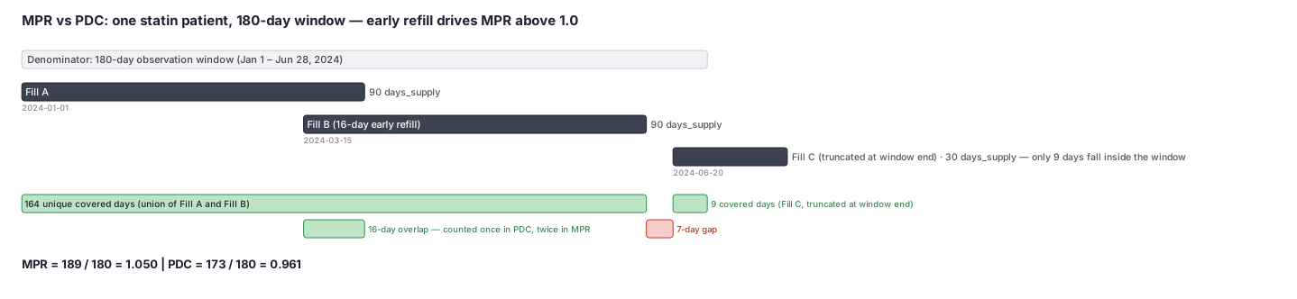
Imagine a patient, ID 2001, who starts a 180-day statin treatment window on January 1, 2024. The pharmacy records show three fills: a 90-day fill picked up at the start, another 90-day fill picked up on March 15 (sixteen days before the first fill runs out — an early refill), and a smaller 30-day fill picked up on June 20. The window closes on June 28 (day 180). We want to compute the MPR and compare it to what PDC would give. The early refill is the key: those sixteen overlapping days are counted once in PDC but counted twice in MPR's simple sum.

Dataset

Raw pharmacy claims rows for patient 2001 — exactly what an analyst pulls from a pharmacy table. The days_supply on Fill C extends past the window end (June 28), so only 9 days count toward the denominator.

Steps

• Set the observation window: 180 days, January 1 through June 28, 2024 (31 + 29 + 31 + 30 + 31 + 28 = 180 days; 2024 is a leap year).

• Fill A (Jan 1, 90 days): covers January 1 through March 30 — fully inside the window; contributes 90 days to the MPR numerator.

• Fill B (Mar 15, 90 days): covers March 15 through June 12 — fully inside the window; contributes 90 days to the MPR numerator. Notice that March 15–30 (16 days) overlaps with Fill A; MPR counts those 16 days again without adjustment.

• Fill C (Jun 20, 30 days): would cover June 20 through July 19, but the window ends June 28, so only the 9 days June 20–28 fall inside; contributes 9 days to the MPR numerator (the remaining 21 days are truncated at the window boundary).

• MPR numerator = 90 + 90 + 9 = 189 days of supply within the window.

• MPR = 189 / 180 = 1.050 — the early refill pushed the ratio above 1.0.

• For contrast, PDC merges Fill A and Fill B into a single covered block: January 1 through June 12 = 164 unique days (the 16-day overlap is counted once, not twice). Then a 7-day gap (June 13–19), then Fill C adds 9 more unique days (June 20–28). Unique covered days = 164 + 9 = 173. PDC = 173 / 180 = 0.961.

• The gap between the two measures (MPR 1.050 vs PDC 0.961) is produced entirely by the 16-day early refill overlap: MPR double-counts those 16 days; PDC does not.

Result

Label

MPR = 189 days_supply in window / 180 window days = 1.050 (above the 0.80 adherent threshold, and above 1.0 due to the 16-day overlap). PDC = 173 unique covered days / 180 window days = 0.961. Both measures classify this patient as adherent, but only MPR can exceed 1.0 — PDC is bounded.

Value

1.05

Timeline Spec

Title

MPR vs PDC: one statin patient, 180-day window — early refill drives MPR above 1.0

Caption

Fill B arrives 16 days before Fill A is exhausted (early refill). MPR sums all supply including the overlap (189 / 180 = 1.050); PDC merges overlapping days so each calendar day counts once (173 / 180 = 0.961). The shaded overlap band is the entire wedge between the two measures.

Alt Text

Horizontal timeline from 2024-01-01 to 2024-06-28 showing three fill bars. Fill A (Jan 1, 90 days) and Fill B (Mar 15, 90 days) overlap from Mar 15 to Mar 30 — that overlap region is highlighted. A 7-day gap runs Jun 13–19. Fill C (Jun 20) is truncated at the window end on Jun 28. An underlay shows 164 covered days merged from Fills A and B, a gap, and 9 days from Fill C; the result label shows MPR 1.050 and PDC 0.961.

Window

Start

2024-01-01

End

2024-06-28

Label

Denominator: 180-day observation window (Jan 1 – Jun 28, 2024)

Events

• Label

  Fill A

  Start

  2024-01-01

  Length Days

  90

  Quantity

  90 days_supply

• Label

  Fill B (16-day early refill)

  Start

  2024-03-15

  Length Days

  90

  Quantity

  90 days_supply

• Label

  Fill C (truncated at window end)

  Start

  2024-06-20

  Length Days

  30

  Quantity

  30 days_supply — only 9 days fall inside the window

Spans

• Kind

  covered

  Start

  2024-01-01

  End

  2024-06-12

  Label

  164 unique covered days (union of Fill A and Fill B)

• Kind

  overlap

  Start

  2024-03-15

  End

  2024-03-30

  Label

  16-day overlap — counted once in PDC, twice in MPR

• Kind

  gap

  Start

  2024-06-13

  End

  2024-06-19

  Label

  7-day gap

• Kind

  covered

  Start

  2024-06-20

  End

  2024-06-28

  Label

  9 covered days (Fill C, truncated at window end)

Result

Label

MPR = 189 / 180 = 1.050 | PDC = 173 / 180 = 0.961

Value

1.05

Runnable example

import pandas as pd
import numpy as np

WINDOW_DAYS = 180  # fixed observation interval anchored at the first fill

def compute_mpr(fills: pd.DataFrame, window_days: int = WINDOW_DAYS) -> pd.DataFrame:
    f = fills.sort_values(["person_id", "fill_date"]).copy()

    # Index = first qualifying fill; window = [index_date, index_date + window_days).
    f["index_date"] = f.groupby("person_id")["fill_date"].transform("min")
    f["window_end"] = f["index_date"] + pd.to_timedelta(window_days, unit="D")
    f = f[(f["fill_date"] >= f["index_date"]) & (f["fill_date"] < f["window_end"])]

    # Truncate each fill's supply at the window end (no credit for supply past the window).
    f["supply_end"] = f["fill_date"] + pd.to_timedelta(f["days_supply"], unit="D")
    capped_end = np.minimum(f["supply_end"].values, f["window_end"].values)
    f["days_in_window"] = (capped_end - f["fill_date"].values) / np.timedelta64(1, "D")
    f["days_in_window"] = f["days_in_window"].clip(lower=0)

    # (1) Simple uncapped MPR = sum(days_supply in window) / window_days.
    simple = (f.groupby("person_id")["days_in_window"].sum() / window_days)

    # (3) Shift-forward MPR: walk fills, push a fill's start to the prior supply-end
    #     so overlapping (early-refill / stockpiled) days are carried forward, not
    #     double-counted. Approximates carry-over PDC.
    def shift_forward(g: pd.DataFrame) -> float:
        cursor = g["index_date"].iloc[0]            # earliest uncovered day
        win_end = g["window_end"].iloc[0]
        covered = 0.0
        for fill_date, ds in zip(g["fill_date"], g["days_supply"]):
            start = max(fill_date, cursor)          # never start before existing supply ends
            end = min(start + pd.Timedelta(days=int(ds)), win_end)
            covered += max((end - start).days, 0)
            cursor = max(cursor, end)
        return covered / window_days

    shifted = f.groupby("person_id", group_keys=False).apply(shift_forward)

    out = pd.DataFrame({"mpr_simple": simple, "mpr_shift_forward": shifted})
    out["mpr_capped"] = out["mpr_simple"].clip(upper=1.0)  # (2) cap at 1.0
    return out.reset_index()

library(data.table)
WINDOW_DAYS <- 180L

compute_mpr <- function(fills, window_days = WINDOW_DAYS) {
  f <- as.data.table(fills)
  setorder(f, person_id, fill_date)

  f[, index_date := min(fill_date), by = person_id]
  f[, window_end := index_date + window_days]
  f <- f[fill_date >= index_date & fill_date < window_end]

  # Truncate supply at window end -> days actually inside the fixed window.
  f[, supply_end := fill_date + days_supply]
  f[, days_in_window := pmax(0L, as.integer(pmin(supply_end, window_end) - fill_date))]

  # (1) Simple uncapped MPR.
  simple <- f[, .(mpr_simple = sum(days_in_window) / window_days), by = person_id]

  # (3) Shift-forward MPR: carry overlapping supply forward instead of double-counting.
  shift_one <- function(fd, ds, idx, wend) {
    cursor <- idx; covered <- 0L
    for (i in seq_along(fd)) {
      start <- max(fd[i], cursor)
      end   <- min(start + ds[i], wend)
      covered <- covered + max(as.integer(end - start), 0L)
      cursor  <- max(cursor, end)
    }
    covered / window_days
  }
  shifted <- f[, .(mpr_shift_forward = shift_one(fill_date, days_supply,
                                                 index_date[1], window_end[1])),
               by = person_id]

  out <- merge(simple, shifted, by = "person_id")
  out[, mpr_capped := pmin(mpr_simple, 1.0)]   # (2) cap at 1.0
  out[]
}