Landmark Analysis

In plain language

When researchers want to compare cancer patients who responded to treatment versus those who did not, they face a hidden trap: responders had to survive long enough to be classified as responders, giving them a head-start advantage that has nothing to do with the treatment. A fixed-point analysis fixes this by choosing a specific calendar day — say, day 90 after diagnosis — and asking only: who was still alive and event-free on that day, and did they respond before it? Everyone who died or had their outcome before day 90 is set aside, the groups are locked in based only on what happened before day 90, and survival tracking begins fresh from day 90 onward. This gives each group a fair start and measures how long patients lived *after* the classification moment, not from a zero point that secretly favors one group.

Landmark analysis

answers a conditional question in time-to-event data: among subjects who are still alive, event-free, and under observation at a fixed clock time (the landmark), what is the outcome hazard contrasted by an exposure or response status that is fully determined by that landmark? The defining mechanic is a deliberate realignment of the time axis. You (1) choose a landmark time `L` from clinical knowledge of when the classifying event is observable (e.g., 90 days after a cancer diagnosis, 30 days after an MI hospitalization), (2) discard everyone who has the outcome, dies, or is censored before `L`, (3) freeze exposure status using only data accrued in `[index, L]`, and (4) start the outcome clock at `L` (`follow_up = event_date - L`). A standard Cox model, Kaplan-Meier curve, or Fine-Gray competing-risks model is then fit on the landmark-conditional cohort.

Core estimand distinction

Landmark estimates the exposure-outcome contrast conditional on being event-free and observable at the landmark, with exposure as known by the landmark — it is not a marginal effect from time zero, and it is not the same estimand as the alternatives it is usually compared with. A time-dependent (extended) Cox model (see standard-cox-time-dependent) uses all person-time and lets exposure accrue as a time-varying covariate, so pre-landmark person-time is retained and the at-risk set is never truncated; it estimates an instantaneous-hazard contrast across the whole follow-up. Clone-censor-weight / g-methods (see marginal-structural-models-g-methods) assign every subject to treatment strategies at baseline, censor at the moment they deviate, and weight for the resulting informative censoring, targeting a strategy contrast under sustained regimens. Landmark is the simplest of the three but answers the narrowest question: it conditions on survival to `L` and therefore changes both the population (landmark survivors) and the time origin. The competing-risks estimand must also be pre-specified — a cause-specific hazard (PROC PHREG / coxph) answers an etiologic question, while a subdistribution hazard / cumulative incidence (Fine-Gray) answers an absolute-risk question; the two diverge whenever competing mortality differs by exposure (see competing-risks-cause-specific-fine-gray-rwe).

Pros, cons, and trade-offs

- vs naive "ever exposed / ever responder" from time zero: the naive contrast gives exposed/responder subjects credit for the immortal time they had to survive in order to become exposed — pure guarantee-time bias that manufactures an apparent benefit. Landmark removes it by construction (no one can be classified before they have survived to `L`). Prefer landmark whenever exposure or response is defined after follow-up begins and a simple, transparent fix is wanted. - vs time-dependent (extended) Cox: landmark is trivial to specify, communicate, and audit, and it sidesteps the proportional-hazards-of-a-time-varying-covariate assumption. Cost: it throws away all pre-landmark person-time and every subject who fails before `L`, so it is less efficient and the estimate is sensitive to the (arbitrary) choice of `L`. Prefer time-dependent Cox when efficiency matters, when exposure changes repeatedly, or when no single clinically meaningful landmark exists; prefer landmark when the scientific question is genuinely conditional ("among patients alive and responding at 90 days...") or as a transparent sensitivity check on a time-dependent model. - vs clone-censor-weight / g-methods: landmark cannot represent dynamic, sustained, or grace-period strategies and does not handle treatment-confounder feedback. Prefer g-methods for those estimands; prefer landmark for a one-time classification at a fixed point.

When to use

Post-baseline exposure or response classification (tumor response, time-to-initiation, transplant, biomarker conversion) where the contrast must be made fair for the survival required to be classified; oncology and cardiology RWE; as a pre-specified sensitivity analysis alongside a time-dependent Cox primary. The landmark must be chosen on clinical/biological grounds and pre-specified — never data-driven (peeking at outcomes to pick `L` inflates type-I error). Always report results across a grid of landmarks (e.g., 30/60/90/180 days) so reviewers see the dependence on `L`, and frame the estimate explicitly as conditional on landmark survival.

When NOT to use — and when it is actively misleading or dangerous

- Most events occur before a defensible landmark. If the outcome is fast (e.g., 30-day mortality) and `L` is large, you discard most events and the surviving cohort is a thin, selected slice — the estimate may be precise nonsense. - Strong selection on survival-to-landmark. Conditioning on event-free survival to `L` can open a collider path: if an unmeasured factor causes both early events and the exposure, the landmark cohort is differentially depleted by exposure and the conditional contrast is confounded even if time zero was clean. This is dangerous precisely because landmark looks like it has solved the bias problem. - Procedure- or response-anchored time zero without an eligibility anchor. If you set the index (not just the landmark) at the procedure/response itself, you re-import immortal time through the back door — pair landmark with an eligibility-based time zero (diagnosis, hospitalization). - Repeatedly changing exposure. A single landmark freezes a status that genuinely varies; the frozen classification misattributes later person-time. Use a time-dependent or sequential/dynamic landmark approach instead. - Data-driven landmark selection to maximize a hazard ratio — this is `p`-hacking with a survival curve.

Data-source operational depth

- Claims (FFS vs MA): the landmark denominator ("event-free and observable at `L`") is only valid where claims are complete. Medicare Advantage and capitated/bundled person-time drop fee-for-service claims, so a subject can look event-free at `L` simply because their event was never billed to the FFS system — misclassifying the at-risk set. Require continuous A/B (and D if exposure is a drug) FFS enrollment from index through `L` and exclude MA-only person-time. Exposure-by-landmark uses pharmacy (`fill_date`, `days_supply`) or procedure codes accrued in `[index, L]`; sample fills, 90-day mail order, and free samples distort `days_supply` and the inferred initiation date. Differential competing-risk death by exposure is a specific trap in elderly claims: if the sicker arm dies before `L`, the landmark cohort is selectively healthier in that arm — run a Fine-Gray / CIF check, not just cause-specific Cox. - EHR: response and biomarker capture cluster at clinic visits, so the true classifying event may sit just on either side of `L`. Either snap the landmark to the visit grid or use last-observation-carried-forward and document it; do not pretend daily resolution you do not have. Loss-to-system before `L` (patient leaves the network) is informative censoring of the landmark denominator, not random. - Registry: event and treatment timing are high quality, but response/outcome adjudication lags — choose `L` after the adjudication cutoff so you are not classifying on an artificially undercounted event set. Registries typically lack full pharmacy exposure; link to claims to confirm initiation dates within `[index, L]`. - Linked claims-EHR-registry: the ideal substrate (EHR/registry severity + claims completeness + a death index to firm up the competing-risk and at-risk sets), but linkage selects the linkable subset and creates order/fill/service date discrepancies that must be reconciled before `index` and `L` are assigned.

Worked claims example

Question: does early statin initiation after acute MI reduce 1-year recurrent MI, and is the naive "ever-statin" estimate inflated by immortal time? Cohort: adults with an index AMI hospitalization (`index_date` = discharge), ≥365 days of continuous FFS A/B/D enrollment before index (so washout and baseline are observed), and FFS-observable person-time through the landmark. Landmark `L` = 90 days post-discharge. Exposure is classified using only fills in `[index_date, index_date + 90]`: a subject is an early initiator if any statin `fill_date` falls in that window (confirm `days_supply` ≥ 30 to exclude one-off samples). Apply the landmark restriction: drop anyone with the outcome (recurrent MI), death, or disenrollment on or before day 90 — they cannot contribute to a 90-day-conditional contrast. Reset the clock: outcome follow-up time = `event_date - (index_date + 90)`, starting at zero on day 90, censoring at recurrent MI, death (competing risk), disenrollment, or 365 days post index. Fit a cause-specific Cox (early vs late/non-initiator) for the etiologic HR and a Fine-Gray model for the cumulative-incidence contrast, because post-MI mortality is a strong competing risk that differs by statin use. Then show the bias: re-run the naive analysis that counts statin status as "ever in the year" from time zero (day 0) and contrast the hazard ratio — the naive HR is biased toward benefit because early initiators had to survive ~90 days to be classified. Finally, repeat the landmark fit at `L` = 30, 60, 180 days as the pre-specified sensitivity grid and report all four, because the conditional population shifts with `L`.

Interpreting the output

A 6-month (180-day) landmark analysis of treatment responders vs non-responders returns: conditional overall survival at 12 months post-landmark = 74% (responders) vs 52% (non-responders), estimated among patients event-free at the landmark.

Formal interpretation. At the landmark time L = 180 days, the cohort is restricted to patients who have not yet experienced the outcome; time is reset to zero from that landmark, and survival is estimated from L onward. The 74% vs 52% comparison is a conditional estimate describing survival from month 6 to month 12 among the subset who reached month 6 event-free. Responder status is classified at or before L, so exposure is time-fixed within the landmark-defined subcohort. This eliminates the immortal-time advantage that responders would otherwise inherit in a time-zero-anchored analysis — but the estimate is conditional on surviving to L and is therefore not marginal from treatment initiation.

Practical interpretation. Landmark analysis answers: "For patients who made it to 6 months without an event, does responding to therapy predict better outcomes thereafter?" This conditional framing is appropriate for prognostic labeling discussions and post-hoc responder analyses, but must be distinguished from the intention-to-treat estimate of overall survival from the start of treatment. Report the N at landmark, the 95% CI for each arm, and sensitivity analyses at pre-specified alternative landmark times.

Worked example

Scenario

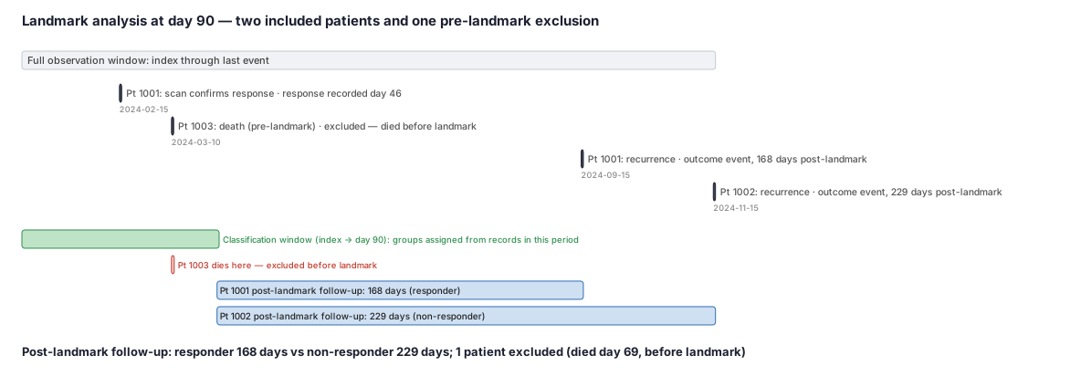
Three lung cancer patients are diagnosed on January 1, 2024 (their index date). Researchers want to know whether patients whose tumors shrank by day 90 live longer afterward than those whose tumors did not. The landmark day is March 31, 2024 — exactly 90 days after index. Scan results and vital status are checked on that day. Only patients alive and recurrence-free on March 31 enter the comparison; their follow-up clock starts fresh on that date.

Dataset

One row per patient showing scan result (recorded during the classification window), vital status at the landmark, and the recurrence date used to compute follow-up time.

Steps

• Set the landmark day: index date January 1 plus 90 days = March 31, 2024.

• Check each patient's vital status and outcome status on March 31: patient 1001 is alive and recurrence-free — keep; patient 1002 is alive and recurrence-free — keep; patient 1003 died on March 10, which is before the landmark — exclude by design.

• Lock each remaining patient's group using only records from January 1 through March 31: patient 1001 had a scan showing tumor shrinkage on February 15 (day 46), so they are in the 'responded' group; patient 1002 had no qualifying response scan before March 31, so they are in the 'did not respond' group.

• Reset the follow-up clock to zero at March 31 for both included patients: patient 1001 has their recurrence on September 15, giving 168 days of follow-up (April = 30, May = 31, June = 30, July = 31, August = 31, September 1–15 = 15 days; total = 168); patient 1002 has their recurrence on November 15, giving 229 days of follow-up (add October = 31 and November 1–15 = 15 days to the 183 days through September 30; total = 229).

• Both patients have the outcome (recurrence), so neither is censored in this small example; in a real study, patients still event-free at the end of the observation window would be censored at that point.

• The contrast is now fair: both responder and non-responder entered the risk set on the same calendar day (March 31), and no one's pre-landmark survival is counted as post-landmark follow-up.

Result

Label

Responder (patient 1001): 168 days to recurrence from landmark. Non-responder (patient 1002): 229 days to recurrence from landmark. Patient 1003 excluded (died before landmark day 90). Analysis is conducted only on the 2 patients event-free at day 90, with follow-up measured from day 90 forward.

Value

168 days (responder) vs 229 days (non-responder) post-landmark follow-up; 1 patient excluded pre-landmark

Timeline Spec

Title

Landmark analysis at day 90 — two included patients and one pre-landmark exclusion

Window

Start

2024-01-01

End

2024-11-15

Label

Full observation window: index through last event

Events

• Label

  Pt 1001: scan confirms response

  Start

  2024-02-15

  Length Days

  1

  Quantity

  response recorded day 46

• Label

  Pt 1003: death (pre-landmark)

  Start

  2024-03-10

  Length Days

  1

  Quantity

  excluded — died before landmark

• Label

  Pt 1001: recurrence

  Start

  2024-09-15

  Length Days

  1

  Quantity

  outcome event, 168 days post-landmark

• Label

  Pt 1002: recurrence

  Start

  2024-11-15

  Length Days

  1

  Quantity

  outcome event, 229 days post-landmark

Spans

• Kind

  exposed

  Start

  2024-01-01

  End

  2024-03-31

  Label

  Classification window (index → day 90): groups assigned from records in this period

• Kind

  gap

  Start

  2024-03-10

  End

  2024-03-10

  Label

  Pt 1003 dies here — excluded before landmark

• Kind

  followup

  Start

  2024-03-31

  End

  2024-09-15

  Label

  Pt 1001 post-landmark follow-up: 168 days (responder)

• Kind

  followup

  Start

  2024-03-31

  End

  2024-11-15

  Label

  Pt 1002 post-landmark follow-up: 229 days (non-responder)

Landmark Marker

Date

2024-03-31

Label

LANDMARK — day 90. Groups locked. Follow-up clock resets to zero. Pre-landmark deaths excluded.

Result

Label

Post-landmark follow-up: responder 168 days vs non-responder 229 days; 1 patient excluded (died day 69, before landmark)

Value

168

Caption

Timeline for three patients with a day-90 landmark. The shaded band (January 1 – March 31) is the classification window: scan results recorded here determine each patient's group. The vertical marker at March 31 is the landmark itself — follow-up for the two surviving patients begins here. Patient 1003, who died on March 10 (before the landmark), is excluded; their pre-landmark time is never counted as post-landmark risk, removing the guarantee-time trap.

Alt Text

Horizontal timeline from January 1 to November 15, 2024. A shaded classification band runs from January 1 to March 31. A vertical line marks the day-90 landmark on March 31. Patient 1001 has a response event on February 15 and a recurrence on September 15, with a follow-up bar from the landmark to that recurrence labeled 168 days. Patient 1002 has no response event and a recurrence on November 15, with a follow-up bar from the landmark labeled 229 days. Patient 1003 has a death marker on March 10, before the landmark, with a label indicating exclusion.

Runnable example

import pandas as pd
from lifelines import CoxPHFitter

def landmark_cox(df: pd.DataFrame, landmark_days: int) -> CoxPHFitter:
    L = df["index_date"] + pd.Timedelta(days=landmark_days)

    # (1) Keep only subjects EVENT-FREE and OBSERVABLE at the landmark.
    #     Anyone with the outcome/death/disenrollment on or before L is excluded by design.
    at_risk = (df["event_date"] > L) & (df["obs_end"] >= L)
    lm = df.loc[at_risk].copy()
    lm["L"] = L[at_risk]

    # (2) Freeze exposure using ONLY information available by the landmark.
    lm["early_exposed"] = (lm["expose_date"].notna() & (lm["expose_date"] <= lm["L"])).astype(int)

    # (3) Reset the time origin to the landmark; follow-up starts at 0 on day L.
    lm["fu_time"] = (lm["event_date"].clip(upper=lm["obs_end"]) - lm["L"]).dt.days
    lm["cs_event"] = (lm["event"] == 1).astype(int)   # cause-specific: competing death treated as censored
    lm = lm[lm["fu_time"] > 0]

    # (4) Cause-specific Cox on the landmark-conditional cohort.
    model = CoxPHFitter()
    model.fit(lm[["fu_time", "cs_event", "early_exposed"]],
              duration_col="fu_time", event_col="cs_event")
    return model

# Pre-specified landmark sensitivity grid (report all; never pick the landmark from the results).
for L_days in (30, 60, 90, 180):
    m = landmark_cox(df, L_days)
    hr = m.hazard_ratios_["early_exposed"]
    print(f"landmark={L_days}d  n={m.event_observed.shape[0]}  HR={hr:.2f}")

library(survival)
library(cmprsk)

landmark_fit <- function(df, landmark_days) {
  L <- df$index_date + landmark_days

  # (1) Subset to subjects event-free and observable at the landmark.
  keep <- df$event_date > L & df$obs_end >= L
  lm <- df[keep, ]
  Lk <- L[keep]

  # (2) Exposure frozen using only [index, L].
  lm$early_exposed <- as.integer(!is.na(lm$expose_date) & lm$expose_date <= Lk)

  # (3) Reset the clock to the landmark.
  lm$fu_time  <- as.numeric(pmin(lm$event_date, lm$obs_end) - Lk)
  lm$cs_event <- as.integer(lm$event == 1L)            # cause-specific endpoint
  lm <- lm[lm$fu_time > 0, ]

  # (4a) Cause-specific Cox (etiologic HR) on the landmark cohort.
  cs <- coxph(Surv(fu_time, cs_event) ~ early_exposed, data = lm)

  # (4b) Fine-Gray subdistribution model (absolute-risk view; competing death = code 2).
  fg <- crr(ftime = lm$fu_time, fstatus = lm$event,
            cov1 = lm[, "early_exposed", drop = FALSE],
            failcode = 1L, cencode = 0L)
  list(n = nrow(lm), cox_hr = exp(coef(cs)), fg_shr = exp(fg$coef))
}

# Pre-specified landmark grid; report every landmark, do not data-mine L.
for (Ld in c(30, 60, 90, 180)) {
  r <- landmark_fit(df, Ld)
  cat(sprintf("landmark=%dd  n=%d  csHR=%.2f  fgSHR=%.2f\n",
              Ld, r$n, r$cox_hr, r$fg_shr))
}