Exposure Lag, Induction, and Latency Windows

In plain language

When a drug is prescribed, there is a short period right after the prescription where any disease event was probably already brewing before the drug could have caused it — so researchers deliberately skip that early window and start counting only after it ends; this skipped window is called the lag period. Beyond the lag, there is also a minimum biological delay — the induction period — before a drug can actually cause a disease event, so events happening too soon after a prescription start are not counted as caused by the drug. A third parameter, the latency period, accounts for the gap between when a disease actually begins in the body and when it shows up in a medical record or database. Together, these three time rules help researchers count only the events that could genuinely have been caused by the drug, rather than events that were already happening for other reasons.

Exposure lag, induction, and latency windows

are the three distinct time parameters that translate a raw exposure date (a pharmacy `fill_date`, an `index_date`, a procedure date) into the calendar interval during which that exposure could plausibly cause and during which an outcome could plausibly be detected. They are routinely conflated, but they are biologically and operationally separable, and confusing them produces some of the most common self-inflicted biases in pharmacoepidemiology. The parameters belong in the protocol estimand and code list before any programming, because each one changes who is at risk, when person-time accrues, and which events are counted.

Core conceptual distinction

— three parameters, three different jobs. (1) Lag (exclusion / blanking) period: a span of follow-up immediately after exposure start during which outcomes are not attributed to the exposure. Its purpose is to remove protopathic bias / reverse causation — the outcome (or its prodrome) was already brewing and caused the prescription, so the drug looks falsely associated (Tamim 2007). Operationally, a lag drops the first L days of follow-up. (2) Induction period: the minimum biological time that must elapse between a causal exposure and the outcome it can produce; exposure occurring within the induction interval before an event cannot have caused that event and should not count as etiologically relevant exposure (Rothman 1981). Operationally, induction shifts the start of the at-risk window forward — current exposure status is `[exposure_start + induction, ...]`. (3) Latency period: the time from biological effect onset to clinical detection/recording; long latency means an event recorded today maps to exposure years ago, so latency widens the relevant exposure lookback (e.g., unopposed estrogen and endometrial cancer require a multi-year window). The estimand distinction matters: with a lag you are estimating a per-protocol effect on outcomes that can be caused after the blanking window; with an induction window you are testing a specific etiologic hypothesis (effects only appear after a minimum delay); the two are not interchangeable, and a misspecified induction window biases toward the null exactly as a misspecified lag biases away from it.

Pros, cons, and trade-offs

- vs no time-window adjustment (raw exposure = at-risk on the fill date): Lag/induction/latency rules remove protopathic bias and biologically implausible "instant-cause" attributions that an unadjusted current-use definition builds in. Cost: they discard person-time and events, reducing power, and every threshold is a judgment call that must be defended and varied in sensitivity analysis. Prefer a lag/induction rule whenever reverse causation or a known biological delay is plausible (almost all chronic-disease and oncology questions, and any acute outcome that can prompt the prescription — e.g., GI symptoms before an NSAID, dyspnea before a respiratory drug). - vs immortal-time fixes (the symmetric error): A lag period drops early follow-up to avoid counting events; done carelessly it can re-create immortal time by guaranteeing survival through the lag for those who are classified as exposed, biasing toward benefit (Suissa 2008). The correct implementation applies the lag identically to both arms and to the time axis, not to eligibility. Prefer explicitly modeling the lag as a delayed-entry / left-truncation interval so the immortal interval is excluded from both numerator and denominator. - vs a single fixed window for everything: A one-size window (e.g., "current use = days_supply only") is simple and reproducible but biologically wrong when the cause-effect delay differs from the supply duration. Cost of the nuanced approach: more programming, more diagnostics, and the need to pre-specify induction/latency by hypothesis. Prefer the nuanced rule for regulatory- or HTA-grade safety/effectiveness work; the simple rule may suffice for purely descriptive utilization counts.

When to use

— apply an explicit lag/induction/latency specification when: (a) the outcome can plausibly cause the exposure (protopathic bias) — apply a lag; (b) there is a known minimum biological delay from exposure to effect — apply an induction window; (c) the disease has a long detectable-preclinical phase or long etiologic latency (cancers, fibrosis, cumulative-dose toxicities) — widen the exposure lookback to the latency horizon; (d) you are building a regulatory-grade comparative safety study where a reviewer (FDA Sentinel, EMA) will probe whether early events are reverse-causation artifacts. In all cases pre-specify the primary window and a grid of sensitivity windows.

When NOT to use — and when it is actively misleading or dangerous

- Acute, immediate-onset effects (anaphylaxis, acute injection-site reaction, hypoglycemia, day-1 bleeding from an anticoagulant). Imposing an induction lag here removes the very events the drug causes and biases toward the null. Do not lag an outcome whose causal mechanism is immediate. - Using a lag to "clean up" a noisy signal without a reverse-causation rationale. A lag chosen post hoc to make a safety signal disappear is data dredging; the lag must be motivated by biology and fixed in the protocol. - Lag applied to eligibility rather than to the time axis. Requiring patients to survive (and stay enrolled) through the lag to be "exposed" manufactures immortal time and a spurious protective effect (Suissa 2008). This is the most dangerous failure mode. - Long-latency cancer outcomes with short data windows. If the database covers 2–3 years but the etiologic latency is 5–15 years, you cannot capture the relevant exposure; the study is uninformative and a non-null finding is more likely contamination (recent exposure, surveillance bias) than a true late effect.

Data-source operational depth

- Claims (FFS): Exposure is the pharmacy fill (`fill_date` + `days_supply`); the at-risk window is `[fill_date + lag_days, fill_date + days_supply + carryover]`, and for an induction hypothesis events within `induction_days` of `fill_date` are not attributed. Failure modes: claim-adjudication lag and reversed claims mean `fill_date` is not the ingestion date; Medicare Advantage (MA)-only person-time lacks fee-for-service claims, so an apparently exposure-free lag interval can be unobserved time rather than true non-exposure — restrict to A/B/D (or commercial medical+pharmacy) enrollees and exclude MA-only spans. Diagnosis dates carry their own coding lag, so a "first GI bleed" date may trail the clinical event, shrinking an apparent protopathic signal. - EHR: Exposure is the order/administration, not the fill, and the outcome is encounter-driven — a long latency window straddles periods where the patient may not have visited, so an event "detected" at a late visit is really an event that occurred earlier (latency is partly a recording artifact here). Confirm starts against linked dispensing; treat between-visit gaps as informative when defining lag follow-up. - Registry: Adjudicated outcomes with clean event dates are a strength (good for induction tests), but registry adjudication lag can correlate with exposure (sicker, more-treated patients are reviewed faster), distorting the apparent induction interval; check whether adjudication date vs event date differs by arm. Registries are usually weak for complete exposure history — link to claims to populate a latency-length lookback. - Linked claims–EHR–vital records: Best substrate for long-latency questions (EHR severity + claims completeness + death index), but order/fill/service-date discrepancies must be reconciled before choosing the exposure anchor, and differential competing risk of death by exposure (common in elderly claims) censors long latency windows unequally — use cause-specific or subdistribution handling rather than naive censoring.

Worked claims example (protopathic lag + induction)

Question: does a newly initiated NSAID raise the rate of hospitalized upper-GI bleed in a commercial + Medicare FFS database? Naive "current use = NSAID days_supply" overcounts because GI discomfort from an existing bleed prompts the NSAID (or its co-prescribed PPI workup), i.e. protopathic bias. Specification: (1) Eligibility: ≥365 days continuous A/B/D (or commercial medical+pharmacy) enrollment before the first NSAID fill (`index_date`); exclude MA-only person-time so the washout and lag are observed, not missing. (2) New-user washout: no NSAID fill in the 365-day lookback. (3) Lag: count person-time and bleed events only from `index_date + 30` (the 30-day blank period removes bleeds that were prodromal to the prescription — Tamim 2007). (4) Exposure window: a fill contributes at-risk time over `[fill_date + 30, fill_date + days_supply + 14]` (14-day carryover/grace for stockpiling); overlapping fills are stitched into a continuous episode. (5) Outcome: first inpatient upper-GI-bleed claim (validated dx in primary position), the event date taken as admission date to limit coding lag. (6) Censor at disenrollment, death, end of data, and exposure-episode end + grace. (7) Sensitivity: rerun with lag = 0, 14, 60, 90 days and report how the rate ratio moves — a signal that only exists at lag 0 is the protopathic-bias fingerprint. Contrast this with a long-latency variant (unopposed estrogen → endometrial cancer): there the relevant change is not a 30-day lag but a multi-year induction window (count exposure 5+ years before the cancer date) and a lookback long enough to capture it — a 2-year claims extract cannot answer that question.

Worked example

Scenario

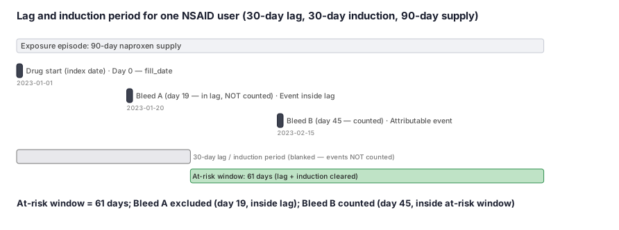
Patient 2001 starts a new NSAID (naproxen) on 2023-01-01 for pain. Researchers want to know whether NSAID use raises the rate of hospitalized stomach bleeding. Because stomach discomfort from an existing bleed can prompt a doctor to prescribe an NSAID in the first place, any bleed recorded in the first 30 days after the prescription is suspicious — it may have been the reason for the prescription, not a consequence of it. The study therefore applies a 30-day lag: follow-up and event counting start on day 31 (2023-01-31). The drug also needs a minimum biological dwell time to cause mucosal damage, so an induction period of 30 days is also applied: the at-risk window does not open until 30 days after the fill date. Because both the lag and the induction period are 30 days here, the at-risk window opens on 2023-01-31. The fill covers 90 days of supply, so the exposure episode runs through 2023-04-01 (day 91). The combined at-risk window is therefore 2023-01-31 to 2023-04-01, a span of 61 days. A bleed recorded on 2023-02-15 falls inside that window and is counted; a bleed recorded on 2023-01-20 falls inside the lag and is not counted.

Dataset

Claims pharmacy and event rows for patient 2001 as an analyst would see them.

Steps

• Fill date is 2023-01-01 (the index date); the 90-day supply means the exposure episode runs from 2023-01-01 through 2023-04-01.

• Apply the 30-day lag: the first 30 days of follow-up (2023-01-01 through 2023-01-30) are blanked out; any event in this window is treated as potentially protopathic and excluded.

• Apply the 30-day induction period: because the lag and induction period are both 30 days and start from the same fill date, the at-risk window opens on the same date — 2023-01-31.

• The at-risk window runs from 2023-01-31 to 2023-04-01, a span of 61 days (31 Jan through 1 Apr inclusive).

• The bleed on 2023-01-20 is on day 19 after the fill — inside the 30-day lag — so it is not attributed to the NSAID.

• The bleed on 2023-02-15 is on day 45 after the fill — past both the lag and the induction period — so it falls inside the at-risk window and is counted as a candidate outcome.

Result

Lagged at-risk window = 2023-01-31 to 2023-04-01 (61 days). The bleed on 2023-01-20 is excluded (inside lag). The bleed on 2023-02-15 is the attributable event: it falls on day 45, which is after the 30-day lag and after the 30-day induction period, inside the 61-day at-risk window.

Timeline Spec

Title

Lag and induction period for one NSAID user (30-day lag, 30-day induction, 90-day supply)

Window

Start

2023-01-01

End

2023-04-01

Label

Exposure episode: 90-day naproxen supply

Events

• Label

  Drug start (index date)

  Start

  2023-01-01

  Length Days

  1

  Quantity

  Day 0 — fill_date

• Label

  Bleed A (day 19 — in lag, NOT counted)

  Start

  2023-01-20

  Length Days

  1

  Quantity

  Event inside lag

• Label

  Bleed B (day 45 — counted)

  Start

  2023-02-15

  Length Days

  1

  Quantity

  Attributable event

Spans

• Kind

  unexposed

  Start

  2023-01-01

  End

  2023-01-30

  Label

  30-day lag / induction period (blanked — events NOT counted)

• Kind

  exposed

  Start

  2023-01-31

  End

  2023-04-01

  Label

  At-risk window: 61 days (lag + induction cleared)

Result

Label

At-risk window = 61 days; Bleed A excluded (day 19, inside lag); Bleed B counted (day 45, inside at-risk window)

Value

61

Caption

After a 30-day lag and 30-day induction period from the 2023-01-01 fill date, the at-risk window opens on 2023-01-31 and closes with the end of the 90-day supply on 2023-04-01. The day-19 bleed falls inside the blanked lag interval and is excluded; the day-45 bleed falls inside the at-risk window and is counted as an attributable event.

Alt Text

Horizontal timeline starting 2023-01-01. A shaded block labeled 30-day lag and induction period covers 2023-01-01 through 2023-01-30, with a marker for Bleed A on 2023-01-20 shown as excluded. An open block labeled at-risk window runs from 2023-01-31 to 2023-04-01, with a marker for Bleed B on 2023-02-15 shown as counted.

Runnable example

import pandas as pd
import numpy as np

LAG_DAYS       = 30   # blank early follow-up to remove protopathic/reverse-causation events (Tamim 2007)
CARRYOVER_DAYS = 14   # stockpiling/grace appended to days_supply
INDUCTION_DAYS = 30   # exposure within this delay before an event cannot have caused it (Rothman 1981)

def build_lagged_exposure(rx: pd.DataFrame, events: pd.DataFrame, fup: pd.DataFrame) -> pd.DataFrame:
    rx = rx.sort_values(["person_id", "fill_date"]).copy()

    # Exposure episode = [fill_date, fill_date + days_supply + carryover]; stitch overlapping fills per person.
    rx["epi_start"] = rx["fill_date"]
    rx["epi_end"]   = rx["fill_date"] + pd.to_timedelta(rx["days_supply"] + CARRYOVER_DAYS, unit="D")
    rx["prev_end"]  = rx.groupby("person_id")["epi_end"].shift().fillna(pd.Timestamp.min)
    rx["new_block"] = (rx["epi_start"] > rx["prev_end"]).astype(int)
    rx["block"]     = rx.groupby("person_id")["new_block"].cumsum()
    epi = (rx.groupby(["person_id", "block"])
             .agg(epi_start=("epi_start", "min"), epi_end=("epi_end", "max"))
             .reset_index())

    # Apply the LAG to the time axis: at-risk follow-up starts at index_date + LAG (delayed entry),
    # so person-time and events in the immortal/protopathic interval are excluded from BOTH num and denom.
    epi = epi.merge(fup, on="person_id", how="inner")
    epi["risk_start"] = np.maximum(epi["epi_start"], epi["index_date"] + pd.Timedelta(days=LAG_DAYS))
    epi["risk_end"]   = np.minimum(epi["epi_end"], epi["fup_end"])
    epi = epi[epi["risk_end"] > epi["risk_start"]]
    epi["person_days"] = (epi["risk_end"] - epi["risk_start"]).dt.days

    # Attribute an event only if it falls in a lagged at-risk window AND >= INDUCTION_DAYS after the contributing fill.
    ev = events.merge(epi, on="person_id", how="inner")
    ev["attributable"] = ((ev["event_date"] >= ev["risk_start"]) &
                          (ev["event_date"] <= ev["risk_end"]) &
                          (ev["event_date"] >= ev["epi_start"] + pd.Timedelta(days=INDUCTION_DAYS)))
    attrib = ev.groupby("person_id")["attributable"].max().astype(int)

    out = (epi.groupby("person_id")["person_days"].sum()
              .to_frame("person_days_at_risk")
              .join(attrib.rename("attributable_event"), how="left").fillna({"attributable_event": 0}))
    return out.reset_index()

library(data.table)
LAG_DAYS <- 30L; CARRYOVER_DAYS <- 14L; INDUCTION_DAYS <- 30L

build_lagged_exposure <- function(rx, events, fup) {
  setDT(rx); setDT(events); setDT(fup)
  setorder(rx, person_id, fill_date)

  # Exposure episodes = [fill_date, fill_date + days_supply + carryover], stitched across overlapping fills.
  rx[, epi_start := fill_date]
  rx[, epi_end   := fill_date + days_supply + CARRYOVER_DAYS]
  rx[, prev_end  := shift(epi_end), by = person_id]
  rx[, new_block := as.integer(is.na(prev_end) | epi_start > prev_end)]
  rx[, block     := cumsum(new_block), by = person_id]
  epi <- rx[, .(epi_start = min(epi_start), epi_end = max(epi_end)), by = .(person_id, block)]

  # Apply lag to the time axis (delayed entry at index_date + LAG); clip to follow-up.
  epi <- merge(epi, fup, by = "person_id")
  epi[, risk_start := pmax(epi_start, index_date + LAG_DAYS)]
  epi[, risk_end   := pmin(epi_end, fup_end)]
  epi <- epi[risk_end > risk_start]
  epi[, person_days := as.integer(risk_end - risk_start)]

  # Event counts only inside a lagged window and at least INDUCTION_DAYS after the contributing fill.
  ev <- merge(events, epi, by = "person_id", allow.cartesian = TRUE)
  ev[, attributable := as.integer(event_date >= risk_start & event_date <= risk_end &
                                  event_date >= epi_start + INDUCTION_DAYS)]
  attrib <- ev[, .(attributable_event = max(attributable)), by = person_id]

  pd <- epi[, .(person_days_at_risk = sum(person_days)), by = person_id]
  merge(pd, attrib, by = "person_id", all.x = TRUE)[is.na(attributable_event), attributable_event := 0L][]
}