Difference-in-Differences with Staggered Adoption

In plain language

Difference-in-differences (DiD) answers the question: did this policy actually cause a change, or would things have shifted anyway? It compares how much an outcome changed before and after a policy in the group affected by the policy, then subtracts the same before-and-after change measured in a group that was not affected — leaving only the part of the change that the policy can take credit for. In real-world evidence it is most useful when an insurer, state, or health system rolls out a new rule (like requiring patients to try a cheaper drug first) and you want to know whether that rule changed prescribing. The method only works if the two groups were trending in the same direction before the policy took effect — a condition you can check but can never fully prove.

Difference-in-differences (DiD)

identifies a causal effect from the differential timing of an intervention across units. The canonical 2x2 estimator takes a treated group and a comparison group, each observed before and after the intervention, and forms ATT = (Y_treated,post - Y_treated,pre) - (Y_control,post - Y_control,pre). Subtracting the comparison group's change purges any time trend common to both groups, so the surviving difference is attributed to the intervention. In RWE this is the workhorse for group-level shocks that individual-level designs cannot exploit: prior-authorization and step-therapy rollouts, formulary tier changes, Medicaid expansion, REMS, value-based contracts, telehealth parity laws, quality-measure thresholds (e.g., PQA/CMS Star measures), and reimbursement reforms.

Core conceptual distinction

— DiD identifies effects from time variation in policy exposure, not from individual treatment choice; this is what separates it from propensity-score, instrumental-variable, and target-trial methods, which exploit cross-sectional variation in who gets treated. Two assumptions do the work and are separable. (1) Parallel trends: absent the intervention, treated and comparison units would have moved in parallel on the additive outcome scale — a counterfactual claim that pre-period data can only fail to refute, never prove. (2) No anticipation: behavior does not change before implementation in response to the future policy (e.g., providers stockpiling fills before a PA rule takes effect). The estimand matters more than novices expect. The 2x2 ATT is a single number; the event-study (dynamic) estimand ATT(e) traces the effect at each lead/lag relative to adoption; the group-time estimand ATT(g,t) (Callaway-Sant'Anna) is the effect for cohort g at calendar time t, and the headline number is an explicit, positively-weighted average of these. The critical RWE pitfall: with staggered adoption (units adopt in different years) and heterogeneous, time-varying effects, the naive two-way fixed-effects (TWFE) coefficient on treated x post is a variance-weighted average of all possible 2x2 comparisons — including "forbidden" comparisons that use already-treated units as controls for later adopters — and can carry negative weights, so it can be the wrong sign even when every unit's true effect is positive (Goodman-Bacon decomposition). Default to group-time/event-study estimators, not TWFE, whenever adoption is staggered.

Pros, cons, and trade-offs

- vs target-trial emulation / active-comparator new-user: DiD shines for system-level interventions (a plan adds PA; a state expands Medicaid) where there is no individual "exposure decision" to emulate and confounding by indication is irrelevant because everyone in a treated unit is exposed. Cost: it answers a policy-level question (effect of the rule, not of taking a drug), needs a credible never/not-yet-treated comparison, and is biased if parallel trends fails. Prefer DiD when the intervention is assigned to groups over time; prefer target-trial/ACNU for individual drug-vs-drug effectiveness. - vs interrupted time series (ITS) / single-group pre-post: DiD adds a comparison group that absorbs secular trends and concurrent shocks (a new guideline, a pandemic) that a single-group ITS would misattribute to the policy. Cost: it requires a comparison group that is actually parallel; a bad control is worse than none. Prefer DiD whenever a plausible unaffected comparison exists. - vs instrumental-variables-pharmacoepi-rwe: Both are quasi-experimental, but DiD leans on parallel trends across units/time while IV leans on instrument relevance and exclusion. Prefer DiD when the natural experiment is a timed policy shock; prefer IV when you have a credible instrument for individual treatment (e.g., preference-based prescribing) but no clean before/after structure. - TWFE vs modern estimators: TWFE is fast and familiar but biased under staggered, heterogeneous effects (negative weighting). Callaway-Sant'Anna, Sun-Abraham (interaction-weighted event study), and de Chaisemartin-D'Haultfoeuille avoid forbidden comparisons. Cost: more covariates/structure and careful choice of never-treated vs not-yet-treated controls. Prefer modern estimators for any staggered design.

When to use

— A discrete intervention is assigned to identifiable units (plans, states, providers, hospitals, counties) at one or more known dates; you can observe outcomes for those units before and after; and you have comparison units that are plausibly subject to the same secular forces but not the intervention. Panel structure (unit-by-period aggregates, or repeated cross-sections with stable composition) is required. Event-study leads should be flat before adoption — inspect them, do not just test them.

When NOT to use — and when it is actively misleading or dangerous

- Parallel trends is implausible and untestable. If treated and comparison units were diverging before the policy (e.g., plans that adopt PA were already cutting utilization), DiD attributes a pre-existing trend to the intervention. Pre-trend non-rejection does NOT license the design — tests are underpowered, and the bias of interest is in the post-period; sensitivity analysis over plausible trend violations (Rambachan-Roth) is the honest answer, not a single placebo p-value. - Naive TWFE under staggered adoption with dynamic effects. This is the dangerous default: the coefficient can flip sign relative to every true unit-level effect because of negative weights and forbidden already-treated comparisons. Using one treated x post coefficient here is a methodological error, not a simplification. - Spillover / SUTVA violation. If the comparison group is contaminated — a multi-state insurer applies a PA rule to all its plans, providers practicing across a state border treat both populations, patients cross contiguous counties, or a "control" formulary carves in the same restriction — the control change embeds a partial treatment effect and DiD is attenuated or reversed. - Compositional change. When the population in a unit changes around the policy (new MA enrollees after an open-enrollment shift, sicker patients churning out), an apparent effect is a risk-mix artifact. Require a balanced panel of units, or model composition explicitly; do not compare unbalanced repeated cross-sections without checking who entered and left. - Anticipation. If behavior shifts before the official start date, the "pre" period is already partly treated; redefine time zero to the announcement or exclude the anticipation window.

Data-source operational depth

- Claims (FFS vs MA): Build a unit-by-month panel (plan-month, state-month, or provider-month) with a stable denominator of continuously enrolled members so the outcome rate is not driven by enrollment churn. The dominant failure mode is Medicare Advantage person-time lacking FFS claims: MA encounter data are incomplete and under-coded relative to FFS, so a panel mixing FFS and MA enrollees will show spurious utilization "drops" wherever MA share rises — restrict the denominator to FFS Parts A/B/D (or a commercial benefit with complete pharmacy capture) and treat MA-only person-time as missing, not zero. Cluster standard errors at the intervention unit (the plan/state), not the patient, because the policy is assigned at the unit level; with few treated clusters (a handful of adopting states), conventional cluster SEs are anti-conservative — use wild cluster bootstrap (Cameron-Gelbach-Miller) or randomization inference. Watch immortal time and differential coding in procedure-based outcomes. - EHR: Site-level documentation and coding behavior can change around a policy (a quality measure incentivizes coding a diagnosis), mimicking a real effect. Include site fixed effects, audit measurement stability across the breakpoint, and prefer outcomes anchored to objective events (labs, dispensings) over problem-list flags. Visit-driven capture means a patient who leaves the system is differentially lost. - Registry: Strong for adjudicated outcomes and severity but typically organized by patient, not by the policy unit; aggregate to the intervention unit and confirm the registry catchment maps cleanly to the treated/control geography. - Linked claims-EHR-vital-records: The ideal substrate (severity + claims completeness + mortality), but linkage selection (only the linkable subset) can differ across treated and control units; verify linkage rates are balanced across the breakpoint before trusting the contrast, and reconcile order/fill/service dates before assigning a period.

Worked claims example

Question: did a commercial plan's introduction of step therapy for branded DPP-4 inhibitors on 2024-01-01 reduce new DPP-4 initiations? Build a plan-month panel. Denominator: members aged >=18 with type 2 diabetes (>=2 diagnoses) and continuous medical + pharmacy enrollment across the month, restricted to FFS-observable benefits (exclude MA-only and capitated person-time so a fill of zero means no fill, not missing data). Outcome rate = new DPP-4 initiations per 1,000 eligible member-months, where a "new initiation" is a DPP-4 NDC fill (`fill_date`) with no DPP-4 fill in the prior 365 days; collapse multiple same-day fills and count first-event per member per episode using `days_supply` to define the look-back. Treated units = plans that imposed step therapy on 2024-01-01; comparison = plans in the same insurer family with no DPP-4 step-therapy change (verified by formulary files, not assumed). For a clean single-date adoption, the 2x2 is ATT = (rate_treated,2024 - rate_treated,2023) - (rate_control,2024 - rate_control,2023). Before trusting it, plot 24 months of leads/lags: the treated and control initiation rates should track in 2022-2023 (parallel pre-trend) with the gap opening only after January 2024. If multiple plans adopted across 2023-2025 (staggered), abandon the single coefficient: fit a Callaway-Sant'Anna group-time ATT using not-yet-treated plans as controls for each adopting cohort, aggregate to a dynamic event-study, and report the simple weighted ATT. Cluster SEs at the plan; with only six treated plans, report a wild cluster bootstrap p-value. Falsification: a negative-control outcome with no plausible link to DPP-4 step therapy (e.g., statin initiation) should show a null ATT; a placebo adoption date in 2022 should show no pre-effect.

Interpreting the output

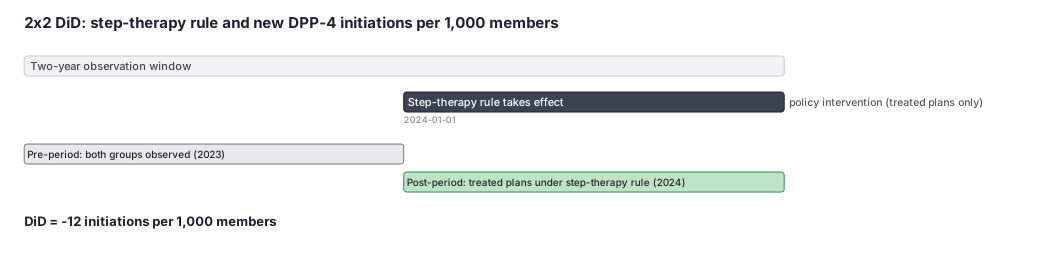
Using the worked example: treated plans had 42 initiations per 1,000 members in 2023 and 28 in 2024 (change = −14); comparison plans moved from 40 to 38 (change = −2). The DiD estimate is (−14) − (−2) = −12 initiations per 1,000 eligible members per year.

Formal interpretation: The DiD estimate of −12 initiations per 1,000 eligible members is the average treatment effect in the treated (ATT) — the portion of the treated plans' post-period decline attributable to the step-therapy rule, after subtracting the secular trend shared by both groups. In staggered-adoption settings where different plans adopt the rule at different calendar times, naive two-way fixed-effects estimation produces a biased ATT because early adopters serve as implicit controls for late adopters, and heterogeneous treatment effects across cohorts can produce negative weights. Callaway-Sant'Anna or Sun-Abraham estimators aggregate group-specific ATTs correctly. The central untestable assumption is parallel trends: absent the policy, treated and comparison plans would have followed the same trajectory. An event-study plot showing no pre-period divergence is necessary — not sufficient — evidence for this assumption.

Practical interpretation: The step-therapy rule is associated with 12 fewer new DPP-4 initiations per 1,000 eligible plan members per year beyond the background decline both groups shared. The 2-unit comparison-group decline captures the secular market trend and is stripped out. This is an intent-to-treat-style policy effect at the plan level and does not reflect the effect on individual patients who found clinical exemptions or other workarounds.

Worked example

Scenario

A commercial health plan added a step-therapy rule for branded DPP-4 inhibitors on 2024-01-01, requiring patients to try a generic first. We want to know whether that rule reduced new DPP-4 initiations. We observe two groups of plans: four plans that adopted the rule (treated) and four comparable plans in the same insurer family that did not (comparison). The outcome is the new-initiation rate per 1,000 eligible members per year. We have one pre-period year (2023) and one post-period year (2024).

Dataset

Plan-year outcome table: new DPP-4 initiations per 1,000 eligible members. Each row is one group-period cell; values are averages across the plans in that group.

Steps

• Compute the treated group change: 28 minus 42 equals negative 14 (the treated plans saw 14 fewer initiations per 1,000 members after the rule).

• Compute the comparison group change: 38 minus 40 equals negative 2 (comparison plans also dropped slightly, capturing the background secular trend).

• Subtract the comparison change from the treated change to remove the secular trend: (negative 14) minus (negative 2) equals negative 12.

• The DiD estimate is negative 12 initiations per 1,000 members — the part of the treated group's drop that the step-therapy rule can take credit for, after stripping out the trend both groups shared.

Result

DiD = (28 - 42) - (38 - 40) = (-14) - (-2) = -12 new initiations per 1,000 eligible members. The step-therapy rule is associated with a reduction of 12 initiations per 1,000 members per year beyond any background trend.

Timeline Spec

Title

2x2 DiD: step-therapy rule and new DPP-4 initiations per 1,000 members

Window

Start

2023-01-01

End

2024-12-31

Label

Two-year observation window

Events

• Label

  Step-therapy rule takes effect

  Start

  2024-01-01

  Length Days

  366

  Quantity

  policy intervention (treated plans only)

Spans

• Kind

  unexposed

  Start

  2023-01-01

  End

  2023-12-31

  Label

  Pre-period: both groups observed (2023)

• Kind

  exposed

  Start

  2024-01-01

  End

  2024-12-31

  Label

  Post-period: treated plans under step-therapy rule (2024)

Result

Label

DiD = -12 initiations per 1,000 members

Value

-12

Runnable example

import pandas as pd
import statsmodels.formula.api as smf
from differences import ATTgt  # pip install differences

panel = panel.copy()
panel["first_treat_period"] = panel["first_treat_period"].fillna(0).astype(int)  # 0 == never treated

# --- Modern staggered estimator: group-time ATT(g,t), never/not-yet-treated controls -----------------
att = ATTgt(data=panel.set_index(["unit_id", "period"]), cohort_name="first_treat_period")
att.fit(formula="outcome_rate", est_method="dr")          # doubly-robust; add covariates via formula RHS
print(att.aggregate("event"))    # dynamic event-study ATT(e): inspect that pre-period leads ~ 0
print(att.aggregate("simple"))   # overall positively-weighted ATT

# --- Naive TWFE for contrast ONLY: biased under staggered timing + heterogeneous effects ------------
panel["treated_post"] = ((panel["first_treat_period"] > 0) &
                         (panel["period"] >= panel["first_treat_period"])).astype(int)
twfe = smf.ols("outcome_rate ~ treated_post + C(unit_id) + C(period)", data=panel).fit(
    cov_type="cluster", cov_kwds={"groups": panel["unit_id"]})
print(twfe.params["treated_post"])  # compare to att.aggregate('simple'); divergence flags TWFE bias

library(did); library(fixest); library(bacondecomp)

# --- Callaway-Sant'Anna group-time ATT with not-yet-treated controls -------------------------------
att <- att_gt(yname = "outcome_rate", tname = "period", idname = "unit_id",
              gname = "first_treat_period", xformla = ~ baseline_rate + region,
              control_group = "notyettreated", clustervars = "unit_id",
              data = panel)
summary(aggte(att, type = "dynamic"))   # event-study: pre-period leads should be ~0 (parallel trends)
summary(aggte(att, type = "simple"))    # overall ATT (positive weights only)

# --- Sun-Abraham interaction-weighted event study (equivalent dynamic estimand) --------------------
es <- feols(outcome_rate ~ sunab(first_treat_period, period) | unit_id + period,
            cluster = ~ unit_id, data = panel[panel$first_treat_period != 1, ])
iplot(es)

# --- Goodman-Bacon: show how the naive TWFE coefficient decomposes (forbidden comparisons) ---------
bgd <- bacon(outcome_rate ~ treated_post, data = panel, id_var = "unit_id", time_var = "period")
print(aggregate(estimate * weight ~ type, data = bgd, FUN = sum))