Normal Distribution and the Central Limit Theorem

In plain language

The normal distribution (the bell curve) describes how averages behave — not how individual patient measurements like costs or hospital stays are shaped, which are almost always right-skewed. The Central Limit Theorem is the reason that t-tests and most regression analyses still work on real-world data: when you average enough patients together, that average follows a bell curve even if each patient's individual value does not. z-scores convert any measurement into "how many standard deviations above or below the group average is this value?" — the standard tool for reporting pediatric growth and laboratory reference ranges.

What the normal distribution is — and what it is not

The normal (Gaussian) distribution is a symmetric, bell-shaped probability distribution with two parameters: mean μ (location) and standard deviation σ (spread). Its probability density function is f(x) = (1 / (σ√2π)) × exp(−(x − μ)² / (2σ²)). The normal is the engine behind z-tests, t-tests, OLS confidence intervals, and Wald-type intervals from logistic regression, Cox models, and GLMs — nearly every inferential tool in the RWE analyst's kit eventually relies on a normal approximation for some sampling distribution.

The critical distinction, missed constantly in applied work, is what exactly follows a normal distribution. It is almost never the raw clinical outcome. Healthcare costs, length-of-stay, prescription counts, biomarker concentrations from right-skewed assays, and time-to-event outcomes are fundamentally non-normal: they are right-skewed, bounded below at zero, or both. This is not a problem to be corrected — it is a property of the data-generating process. The normal distribution is the model for summary statistics computed from samples — specifically means and their differences — not for individual patient values. A distribution of adult heights in a clinic might be approximately normal; the distribution of their total healthcare costs in the same year will not be. Altman and Bland (1995) crystallize this distinction for clinical researchers: a variable need not be normally distributed for its sample mean to be approximately normal. Understanding this gap explains the entire "but costs aren't normal, can I still use a t-test?" question that arises repeatedly in RWE practice.

The normal distribution's shape and the 68-95-99.7 rule

Three properties of the normal distribution that practitioners must have memorized:

1. 68-95-99.7 rule: In a normal distribution with mean μ and SD σ, approximately 68% of observations fall within one σ of μ, 95% within two σ, and 99.7% within three σ. More precisely, the multipliers for exact 95% and 99% probability coverage are 1.96 and 2.576 σ respectively, but the one-two-three mnemonic is reliable for rapid mental calculation. This rule applies to the distribution of individual observations from a normal population; when applied to the sampling distribution of the mean, σ is replaced by the standard error SE = σ/√n — a quantity that shrinks with n, unlike the SD of the raw data.

2. Symmetry: The normal distribution is perfectly symmetric about its mean. Its mean, median, and mode all coincide at μ. For right-skewed outcomes (costs, LOS), the mean exceeds the median, and the mode lies below the median — the symmetry assumption breaks down for raw data, but the CLT rescues the mean as a summary statistic.

3. The standard normal: When X ~ N(μ, σ²), the z-transformation z = (X − μ) / σ produces a standard normal Z ~ N(0, 1). This allows any normal distribution to be converted to one reference distribution for probability calculation. z-scores are the natural language for pediatric growth assessment (WHO HAZ, WAZ, WHZ), educational standardized testing (IQ scales with mean 100 and SD 15), and laboratory reference ranges (the central 95% of a healthy reference population corresponds to the Z ∈ [−1.96, 1.96] interval).

The Central Limit Theorem: precise statement for practitioners

The CLT is one of the most important theorems in applied statistics and is routinely overstated or understated. Precise statement: if X₁, X₂, ..., Xₙ are independent, identically distributed random variables with mean μ and finite variance σ², then the standardized sample mean (X̄ − μ) / (σ/√n) converges in distribution to a standard normal N(0, 1) as n → ∞, regardless of the shape of the underlying distribution. Kwak and Kim (2017) provide a practitioner-focused derivation of this result with biomedical illustrations.

Several practical implications for RWE:

• Rate of convergence depends on skewness. For symmetric distributions the CLT operates at

• The CLT applies to the sampling distribution of the mean, not the raw data. Raw cost

• SE = σ/√n is the key formula. The standard error of the mean shrinks at the rate 1/√n

z-scores, standardization, and the pediatric growth example

A z-score transforms a raw measurement into standard-deviation units relative to a reference: z = (observed value − reference mean) / reference SD. This allows direct comparison across measurements on different scales and provides an immediate probabilistic interpretation via the standard normal: a child with a height-for-age z-score (HAZ) of −2.0 is 2 SDs below the WHO reference median, placing them at approximately the 2.3rd percentile of the reference population (P(Z < −2) ≈ 0.023 from the standard normal CDF). The WHO Multicentre Growth Reference Study established HAZ, WAZ, and WHZ z-scores on reference samples designed to represent optimal growth; studies of pediatric interventions analyze changes in these z-scores — which are normally distributed by construction in the reference population — using standard t-test and regression methods. The same z-score framework underlies DXA T-scores and Z-scores for bone density and educational test score scaling (IQ: mean 100, SD 15 by design).

Why t-tests and OLS are robust at large n — the CLT at work

The t-test and OLS regression both assume that their test statistics follow a t-distribution, which converges to the standard normal for large degrees of freedom. This holds when the outcome is normally distributed, but also — more broadly — when the sample mean is approximately normally distributed. The CLT guarantees the latter for large n regardless of the outcome distribution. This is why a two-sample t-test on healthcare costs with n = 500,000 per arm is asymptotically valid for inference on mean costs, even though the raw cost distribution is severely right-skewed. OLS regression coefficients are linear functions of the outcome and themselves sample means by the Frisch-Waugh theorem; the CLT applies and justifies Wald-based confidence intervals at large n. This is precisely the "Fagerland paradox" noted in parametric-vs-nonparametric-tests: analysts most often reach for nonparametric tests when n is large and non-normality is obvious, but that is the setting where the CLT has already done its work.

Where the CLT fails and alternative methods are required

The CLT does not guarantee valid normal-based inference in every situation:

1. Extreme right tails in cost distributions. Even at n = 100,000, if a tiny fraction of catastrophically expensive patients dominate the mean (costs 50–100× the median), the sample mean is unstable and heavily influenced by those few observations. Inference on the mean via a t-test is technically asymptotically valid, but the estimate may have low effective power and be sensitive to outlier removal choices. Gamma GLMs, two-part models, and bootstrap mean estimation are more appropriate for primary analysis when tail behavior drives the mean estimate.

2. Rare-event proportions near 0 or 1. The normal approximation to a proportion p̂ fails when np < 5 or n(1 − p) < 5. Normal-approximation confidence intervals for rare event rates can produce negative lower bounds, which are nonsensical. Use Clopper-Pearson exact intervals, Wilson score intervals, or likelihood-ratio intervals. This failure mode makes CLT-based z-tests invalid for pharmacovigilance monitoring of very rare adverse events.

3. Small n with heavily skewed outcomes. With n < 20–30 per group and a clearly non-normal outcome (visible on a QQ plot), the CLT has not yet converged. Nonparametric tests (Mann-Whitney, Wilcoxon signed-rank), permutation-based inference, or parametric models suited to the distributional shape (log-normal, gamma) are safer than assuming normality.

4. Sequential safety monitoring with very low expected counts. The maxSPRT and TreeScan methods for sequential drug safety surveillance use exact Poisson likelihoods because the Poisson normal approximation is unreliable when expected event counts per monitoring period are below 5–10. The CLT-protected z-test is not valid in this regime.

Normal approximations to binomial and Poisson — and their breakdown

Two classical normal approximations appear throughout epidemiology and biostatistics:

• Binomial ≈ Normal: If X ~ Bin(n, p), then for large n with np ≥ 5 and n(1 − p) ≥ 5,

• Poisson ≈ Normal: If X ~ Poisson(λ), then for λ ≥ 10–20, X is approximately N(λ, λ).

The breakdown of these approximations is directly relevant to pharmacovigilance. When monitoring for rare adverse events where expected event counts per reporting period may be 0, 1, or 2, the normal approximation fails systematically — it places probability mass at negative counts and produces CIs that are too wide or too narrow depending on the tail of interest. This is the primary reason sequential safety surveillance methods (maxSPRT, the conditional Poisson scan statistic) use exact likelihood-based methods rather than z-score approximations.

QQ plots for normality assessment and why formal normality tests are counterproductive

A quantile-quantile (QQ) plot compares the quantiles of observed data against the theoretical quantiles of a normal distribution. If the data are normal, the points fall on a straight line; curvature indicates departures: an S-shape indicates skewness, a banana shape indicates heavy tails. QQ plots are the appropriate tool for assessing normality in practice.

Formal normality tests — Shapiro-Wilk, Kolmogorov-Smirnov, Anderson-Darling — are actively counterproductive for the following two reasons:

1. Underpowered at small n. At n < 30, Shapiro-Wilk has low power to detect genuine non-normality that would affect inference. The test will accept non-normal data, providing false reassurance precisely when normality matters most for small-sample t-test validity.

2. Overpowered at large n. At n > 500 (and certainly at n > 50,000 typical of claims databases), any trivial departure from normality — a mildly heavy tail, a minor right skew — will produce a highly significant rejection of the normality null (p < 0.001). But that departure may be completely irrelevant to CLT-protected inference on means at that sample size. The test rejects normality because the test is sufficiently sensitive, not because normality matters at that n.

The recommended practice: use a QQ plot to visualize the distributional shape, combine it with subject-matter knowledge about the outcome (costs are always right-skewed; growth z-scores are normal by design; lab values in a reference population are approximately normal by selection), and make the analytical choice on that basis — not on a p-value from a normality test.

Interpreting the output

Consider a pediatric growth study in which 9 infants are measured on a weight-for-age growth index calibrated to a reference population with mean 100 and SD 15. One infant scores 130.

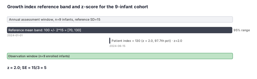
(1) Formal statistical interpretation. The z-score for the infant with index 130 is z = (130 − 100) / 15 = 2.0. Under the reference distribution N(100, 15²), z = 2.0 corresponds to approximately the 97.7th percentile (P(Z < 2.0) ≈ 0.977 from the standard normal CDF). The 68-95-99.7 rule places the interval [100 − 2×15, 100 + 2×15] = [70, 130] as containing approximately 95.4% of the reference population; the infant at 130 sits at the upper edge of this two-SD band. For the sample of 9 infants, the standard error of the mean growth index is SE = 15 / √9 = 15 / 3 = 5 units. A 95% confidence interval for the true population mean among children like those in this sample would be approximately X̄ ± 1.96 × 5, giving a margin of roughly ±9.8 index units. The SD of 15 has not changed — individual children are just as variable as in the reference — but the precision of the group mean has improved by a factor of √9 = 3 compared to knowing only a single child's value.

(2) Practical interpretation. The child with growth index 130 is 2 standard deviations above the reference population average — a value unusual enough (above the 97th percentile of healthy reference children) to warrant clinical documentation, though not extreme enough on its own to indicate pathology. The SD of 15 tells us about how different children are from one another; the SE of 5 tells us how confidently we can estimate the average growth index for the nine children in this clinic visit. In plain language: studying more children narrows our uncertainty about the group average (SE shrinks) but does not reduce child-to-child variability (SD stays around 15).

Pros, cons, and trade-offs

Normal distribution methods (z-tests, t-tests, OLS, normal-based CIs): - Pros: analytically tractable, computationally trivial, directly interpretable effect estimates (mean differences, standardized differences), familiar to all audiences, extensible to regression via OLS, asymptotically valid for inference on means at large n via CLT regardless of raw data distribution shape, exact when the outcome is genuinely normal. - Cons: invalid for inference on extreme quantiles of non-normal outcomes, misleading for rare-event proportions near 0 or 1, slow CLT convergence for extreme right-skew means the approximation may not hold at moderate n with cost-like data, provide no information about distributional shape beyond mean and variance. - When to prefer: inference on means of continuous outcomes with adequate n; z-score comparisons in growth and developmental endpoints where normality holds by design; large-n asymptotic approximation for Wald test statistics from logistic regression, Cox regression, and GLMs; any setting where the estimand is a mean difference.

Normal approximations to binomial and Poisson: - Pros: closed-form test statistics and CIs, computationally fast, excellent approximation when event counts are adequate (np ≥ 5 for binomial; λ ≥ 10 for Poisson). - Cons: fail for rare events, produce nonsensical negative lower bounds for small proportions, invalid for pharmacovigilance with very low expected counts, undercover in the tails. - When to prefer: aggregate count data with common events; background comparisons in large registry analyses; standard rate ratios and relative risks where events are frequent.

QQ plots versus formal normality tests: - QQ plots (prefer): visualize the full distributional shape and departure pattern, scale appropriately across all sample sizes, reveal the type of non-normality (skewness vs heavy tails), do not produce misleading "statistically significant non-normality" in large databases. - Formal tests (avoid as decision gates): counterproductive at both extremes of n; Shapiro- Wilk and Kolmogorov-Smirnov provide a binary signal that conveys less information than a visual QQ plot and should not be used as the gating criterion for parametric vs nonparametric analysis choice.

When to use

Normal distribution methods and CLT-based approximations are appropriate when: - The target of inference is a mean or mean difference, and the CLT is plausible given n and the degree of skew: n ≥ 30–50 per group for mildly skewed continuous outcomes, n ≥ 100+ for moderately skewed, with formal assessment via QQ plot and distributional knowledge. - The outcome is normally distributed by design — pediatric growth z-scores (HAZ, WAZ, WHZ), IQ-type standardized scores, clinical biomarker z-scores referenced against a healthy population — and inference on individual z-scores or mean z-scores is the goal. - Standardization to z-scores is needed for cross-metric comparison across outcomes measured on different scales within a multi-endpoint RWE study. - Normal approximations to binomial or Poisson apply, with np ≥ 5 and n(1 − p) ≥ 5 confirmed. - As the large-n asymptotic approximation justifying Wald confidence intervals reported by standard software from logistic, Cox, and GLM regression procedures.

When NOT to use — and when it is actively misleading or dangerous

• Raw non-normal clinical outcomes analyzed as if individually normal. Fitting a normal model
• Rare-event proportions. If np < 5 or n(1 − p) < 5, the normal approximation to the
• Formal normality testing as a decision gate. Using Shapiro-Wilk as the selector between
• Inference on extreme quantiles of right-skewed distributions. The CLT justifies normal-based
• Small n with clearly non-normal outcomes. With n < 15–20 per group and a distribution
• Sequential safety monitoring with rare events. maxSPRT and similar sequential surveillance

Data-source operational depth

• Claims: With n typically exceeding 100,000 per arm in comparative effectiveness studies,
• EHR: Growth z-scores, laboratory reference values, and vital signs may be approximately
• Registry: Disease severity scores (PRO instruments) are typically bounded and ordinal —
• Primary: Small pilot and interventional studies (n < 50 per arm) are the regime where CLT

Worked example

Scenario

A pediatric endocrinology clinic tracks a weight-for-age growth index calibrated to a reference population with mean 100 and standard deviation 15. A child at today's visit has a growth index of 130, and the team wants to know how many standard deviations above the reference average that child is. Separately, they want to know how precisely the clinic's nine enrolled infants estimate the true mean growth index, expressed as a standard error.

Dataset

Growth index measurements for 9 infants enrolled in the clinic cohort, plus the reference population parameters. The child with index 130 is a single patient whose z-score is computed against the reference mean and SD.

Steps

• Reference parameters: mean = 100, SD = 15. The child of clinical interest has growth index 130, which is above the reference mean.

• z-score = (130 - 100) / 15 = 30 / 15 = 2.0. This child is exactly 2.0 standard deviations above the reference mean, placing them at approximately the 97.7th percentile of the reference population (from the standard normal CDF: P(Z < 2.0) = 0.977).

• The 68-95-99.7 rule tells us that about 95% of the reference population falls in the interval [100 - 215, 100 + 215] = [70, 130]. The child at 130 sits at the upper boundary of the two-standard-deviation reference band.

• For the 9 enrolled infants, we compute the standard error of the mean growth index. The reference SD is 15 and n = 9. Because sqrt(9) = 3, SE = 15 / 3 = 5. The SE is 3 times smaller than the SD, because averaging across 9 patients is 3 times more precise than a single patient measurement.

• The SD of 15 stays fixed — it describes how spread out individual children are around the reference mean. The SE of 5 describes only how precisely we know the mean of this particular group of 9. These are answering different questions.

Result

z = (130 - 100) / 15 = 2.0; the child is at the 97.7th percentile of the reference distribution. SE = 15 / 3 = 5; the 9-infant sample estimates the true mean to within approximately plus or minus 9.8 index units (1.96 times SE). The SD of 15 describes child-to-child variability and does not change with n; the SE of 5 describes precision of the group mean and shrinks as sqrt(n) grows.

Timeline Spec

Title

Growth index reference band and z-score for the 9-infant cohort

Window

Start

2024-01-01

End

2024-12-31

Label

Annual assessment window, n=9 infants, reference SD=15

Events

• Label

  Reference mean band: 100 +/- 2*15 = [70, 130]

  Start

  2024-01-01

  Length Days

  365

  Quantity

  95% range

• Label

  Patient index = 130 (z = 2.0, 97.7th pct)

  Start

  2024-06-15

  Length Days

  1

  Quantity

  z=2.0

Spans

• Kind

  covered

  Start

  2024-01-01

  End

  2024-12-31

  Label

  Observation window (n=9 enrolled infants)

Result

Label

z = 2.0; SE = 15/3 = 5

Value

2.0

Runnable example

import numpy as np
from scipy import stats

# ── Z-score and standard normal lookups ────────────────────────────────────
mu, sigma = 100.0, 15.0    # reference population parameters
x_obs = 130.0              # observed patient value

z = (x_obs - mu) / sigma   # z = (130 - 100) / 15 = 2.0
print(f"z-score: ({x_obs} - {mu}) / {sigma} = {z:.1f}")

p_below = stats.norm.cdf(z)   # P(Z < 2.0) from standard normal CDF
print(f"Percentile: P(Z < {z:.1f}) = {p_below:.4f}  ({p_below*100:.1f}th percentile)")

# pdf: height of the bell curve at z = 2.0
print(f"pdf at z=2.0: {stats.norm.pdf(z):.4f}")

# ppf (quantile function): what z gives the 97.5th percentile?
print(f"97.5th percentile z-score: {stats.norm.ppf(0.975):.4f}  (= 1.96)")

# 68-95-99.7 rule as exact probabilities
for n_sd in [1, 2, 3]:
    lo, hi = mu - n_sd * sigma, mu + n_sd * sigma
    p_inside = stats.norm.cdf(hi, loc=mu, scale=sigma) - stats.norm.cdf(lo, loc=mu, scale=sigma)
    print(f"  [{mu} +/- {n_sd}*{sigma}] = [{lo:.0f}, {hi:.0f}] contains {p_inside*100:.2f}%")

# ── SE shrink: n=9, SE = sigma/sqrt(n) = 15/3 = 5 ─────────────────────────
n = 9
se = sigma / np.sqrt(n)   # 15 / 3 = 5.0
print(f"\nSE = {sigma} / sqrt({n}) = {sigma} / {int(np.sqrt(n))} = {se:.1f}")
print(f"  SD of raw data: {sigma} (unchanged by n)")
print(f"  SE of mean for n={n}: {se:.1f} (shrinks; SD/sqrt(n))")
ci_lo = mu - 1.96 * se
ci_hi = mu + 1.96 * se
print(f"  95% CI for sample mean: [{ci_lo:.2f}, {ci_hi:.2f}]  (margin = {1.96*se:.2f})")

# ── CLT simulation: exponential population -> sample means converge to N ───
# Exponential is strongly right-skewed (skewness = 2); shows CLT in action
rng = np.random.default_rng(42)
pop = rng.exponential(scale=1.0, size=200_000)
pop_skew = stats.skew(pop)
print(f"\nPopulation (exponential): skewness = {pop_skew:.2f}  (strongly right-skewed)")

for n_sample in [2, 10, 30, 100]:
    sample_means = np.array([rng.exponential(scale=1.0, size=n_sample).mean()
                             for _ in range(5_000)])
    skewness = stats.skew(sample_means)
    # Shapiro-Wilk on first 1000 (limit for shapiro); near-normal <-> p > 0.05
    _, p_sw = stats.shapiro(sample_means[:1000])
    label = "near-normal" if p_sw > 0.05 else "still skewed"
    print(f"  n={n_sample:4d}: mean skewness = {skewness:+.3f},  Shapiro-Wilk p = {p_sw:.4f}  ({label})")

# ── QQ plot (requires matplotlib; shows visual normality check) ─────────────
try:
    import matplotlib
    matplotlib.use("Agg")
    import matplotlib.pyplot as plt

    fig, axes = plt.subplots(1, 2, figsize=(10, 4))

    # Raw exponential data: QQ shows systematic curvature (non-normal)
    stats.probplot(pop[:1000], dist="norm", plot=axes[0])
    axes[0].set_title("QQ: exponential raw data\n(S-curve = right-skewed, not normal)")

    # Sample means with n=30: near-straight line (CLT has converged)
    means_30 = np.array([rng.exponential(scale=1.0, size=30).mean()
                          for _ in range(1000)])
    stats.probplot(means_30, dist="norm", plot=axes[1])
    axes[1].set_title("QQ: means of n=30 samples\n(straight line = CLT has converged)")

    plt.tight_layout()
    plt.savefig("qq_clt_demo.png", dpi=100)
    print("\nQQ plots saved to qq_clt_demo.png")
except ImportError:
    print("\n(matplotlib not available; QQ plots skipped)")

# ── Z-score and standard normal (dnorm / pnorm / qnorm) ─────────────────────
mu <- 100.0; sigma <- 15.0; x_obs <- 130.0

z <- (x_obs - mu) / sigma        # z = (130 - 100) / 15 = 2.0
cat(sprintf("z-score: (%.0f - %.0f) / %.0f = %.1f\n", x_obs, mu, sigma, z))

p_below <- pnorm(z)              # P(Z < 2.0); equivalently pnorm(130, mean=100, sd=15)
cat(sprintf("Percentile: P(Z < %.1f) = %.4f  (%.1f-th percentile)\n",
            z, p_below, p_below * 100))

cat(sprintf("pdf at z=2.0: %.4f\n", dnorm(z)))
cat(sprintf("97.5th percentile z-score: %.4f  (= 1.96)\n", qnorm(0.975)))

# 68-95-99.7 rule
for (n_sd in 1:3) {
  lo <- mu - n_sd * sigma; hi <- mu + n_sd * sigma
  p_inside <- pnorm(hi, mean = mu, sd = sigma) - pnorm(lo, mean = mu, sd = sigma)
  cat(sprintf("  [%g +/- %d*%g] = [%g, %g] contains %.2f%%\n",
              mu, n_sd, sigma, lo, hi, p_inside * 100))
}

# ── SE shrink: n=9, SE = sigma/sqrt(n) = 15/3 = 5 ──────────────────────────
n  <- 9L
se <- sigma / sqrt(n)            # 15 / 3 = 5.0
cat(sprintf("\nSE = %.0f / sqrt(%d) = %.0f / %.0f = %.1f\n",
            sigma, n, sigma, sqrt(n), se))
cat(sprintf("  SD of raw data: %.0f  (unchanged by n)\n", sigma))
cat(sprintf("  SE of mean for n=%d: %.1f  (shrinks; SD/sqrt(n))\n", n, se))
ci_lo <- mu - 1.96 * se; ci_hi <- mu + 1.96 * se
cat(sprintf("  95%% CI for sample mean: [%.2f, %.2f]  (margin = %.2f)\n",
            ci_lo, ci_hi, 1.96 * se))

# ── CLT simulation: exponential population -> sample means converge to N ────
set.seed(42)
pop <- rexp(200000, rate = 1)    # strongly right-skewed (skewness = 2)

# skewness function: use e1071 if available, else compute manually
sk_fn <- function(x) {
  m <- mean(x); s <- sd(x)
  mean(((x - m) / s)^3)
}

cat(sprintf("\nPopulation (exponential): skewness = %.2f  (strongly right-skewed)\n",
            sk_fn(pop)))

for (n_sample in c(2L, 10L, 30L, 100L)) {
  sample_means <- replicate(5000, mean(rexp(n_sample, rate = 1)))
  skewness_sm  <- sk_fn(sample_means)
  # Shapiro-Wilk limited to n=5000; use first 1000 for consistency
  sw_p         <- shapiro.test(sample_means[1:1000])$p.value
  label        <- if (sw_p > 0.05) "near-normal" else "still skewed"
  cat(sprintf("  n=%4d: mean skewness = %+.3f,  Shapiro-Wilk p = %.4f  (%s)\n",
              n_sample, skewness_sm, sw_p, label))
}

# ── QQ plots in base R ──────────────────────────────────────────────────────
opar <- par(mfrow = c(1, 2), mar = c(4, 4, 3, 1))

# Raw exponential data: S-curve curvature shows right skew
qqnorm(pop[1:1000], main = "QQ: exponential raw data\n(curvature = not normal)",
       pch = 1, cex = 0.5, col = "grey40")
qqline(pop[1:1000], col = "red", lwd = 2)

# Means of n=30 samples: near-straight line (CLT has converged)
means_30 <- replicate(1000, mean(rexp(30, rate = 1)))
qqnorm(means_30, main = "QQ: means of n=30 samples\n(straight line = CLT converged)",
       pch = 16, cex = 0.6, col = "steelblue")
qqline(means_30, col = "darkblue", lwd = 2)

par(opar)
cat("\nQQ plots displayed. Straight line = normal; curvature = skewed or heavy-tailed.\n")
cat("Use QQ plots for normality assessment, NOT Shapiro-Wilk p-values.\n")