MaxSPRT and Sequential Safety Surveillance

In plain language

MaxSPRT is a way to watch a new drug or vaccine in real time and catch a safety problem as early as the data honestly allow. Every week or month, you count how many times a specific bad event actually happened in the people exposed, and compare it to how many you would expect if the product were harmless. Because you are peeking at the data over and over, a plain "is it significant yet?" test would raise false alarms by chance, so MaxSPRT uses a special threshold designed up front to keep the total false-alarm rate at a fixed level no matter how many times you look. When the running evidence crosses that threshold you declare a signal and investigate - the crossing means the excess is more than the noise of repeated peeking, not that the drug is proven guilty.

Active safety surveillance asks a deceptively simple question and answers it under brutal constraints. The question: is this newly marketed drug, or this season's vaccine, causing an adverse event more often than background? The constraints: you want to know as early as possible (the public-health value of an early signal is enormous), you are looking repeatedly as weekly or monthly data feeds arrive, and every look is another chance to cry wolf. Naive repeated significance testing - run a chi-square each month, signal the first time p < 0.05 - inflates the false-alarm rate without bound: with enough looks you will eventually cross 0.05 by chance even when nothing is wrong. Sequential analysis solves this by designing the stopping rule up front so that the total probability of ever falsely signaling, across all the planned looks, equals a fixed alpha. This is the machinery behind the FDA Sentinel System and the CDC/Vaccine Safety Datalink (VSD) Rapid Cycle Analysis programs.

The MaxSPRT statistic

Wald's classic sequential probability ratio test (SPRT) pits a fixed null (relative risk RR = 1) against a fixed, pre-specified alternative (say RR = 2). Its weakness in surveillance is that you rarely know the true effect size you are hunting; if you guess the alternative wrong, power collapses. Kulldorff et al. (2011) maximize the likelihood ratio over all RR > 1 at each look, removing the need to pre-specify the alternative. For Poisson data the log-likelihood ratio (LLR) at a look with cumulative observed events n and cumulative expected events mu (the count you would see under RR = 1) is, when n > mu, `LLR = n ln(n / mu) + mu - n`, and 0 otherwise. You compute this LLR at every look and signal the first time it crosses a critical boundary (a critical value on the LLR scale). That boundary is not 1.96-anything; it is solved by simulation/recursion so that the chance of the LLR ever* exceeding it during the whole surveillance, under the null, equals alpha (commonly one-sided 0.05). The boundary depends on the maximum length of surveillance (expressed as a maximum expected count, the "sample size") and the look schedule, and it is the device that spends alpha across the looks. MaxSPRT comes in flavors keyed to the comparator: Poisson MaxSPRT when expected counts come from a historical/background rate; binomial MaxSPRT when each case is matched to concurrent comparators so the expected fraction of events falling on the exposed is fixed by the matching ratio; and conditional MaxSPRT (CmaxSPRT) when the historical comparison data are themselves limited and their sampling uncertainty must be folded in.

Group-sequential alternatives

MaxSPRT is, in effect, a continuous-inspection / fully-sequential boundary (look after every event or every tiny batch). The other school is group-sequential monitoring (Pocock, O'Brien-Fleming, or error-spending boundaries of Lan-DeMets type) that tests at a handful of pre-planned analysis times. Group boundaries are more familiar to trialists, are simple to communicate, and concentrate alpha at later looks (O'Brien-Fleming) so an early signal must be very strong; MaxSPRT's flat-ish LLR boundary is tuned for earliest possible detection with many looks. The Cook/Nelson line of work showed these can be unified under an error-spending view, and Sentinel/VSD use both depending on the product and feed cadence.

Interpreting the output

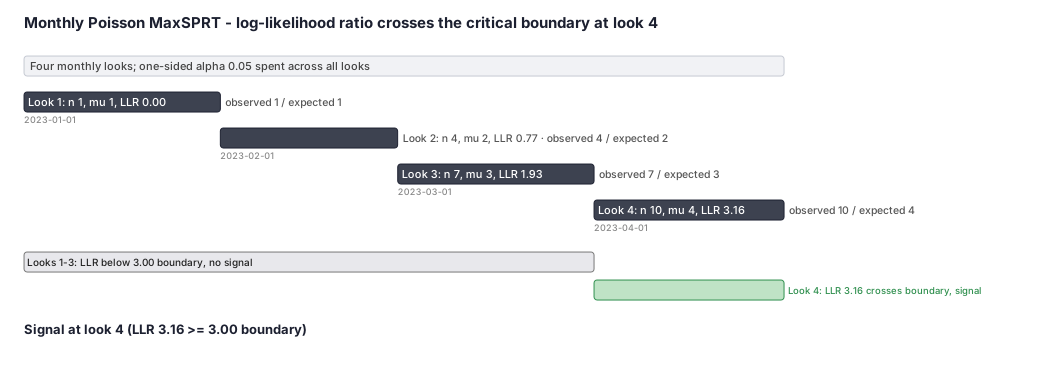
From the worked example: cumulative expected counts mu = 1, 2, 3, 4 at looks 1–4; cumulative observed n = 1, 4, 7, 10. Poisson LLR values: Look 1 = 0, Look 2 ≈ 0.77, Look 3 ≈ 1.93, Look 4 ≈ 3.16. Pre-computed critical boundary ≈ 3.0. Signal is declared at Look 4 (LLR 3.16 ≥ 3.0): observed 10 events vs expected 4.

Formal interpretation: The LLR of 3.16 at Look 4 exceeds the pre-specified sequential boundary of 3.0, declaring a signal. The boundary was computed so that — across all four looks combined — the probability of the LLR ever exceeding it under the true null (RR = 1) is controlled at alpha = 0.05. This is an alpha-spending statement, not a fixed-sample p-value. The LLR crossing does not mean p < 0.05 in the ordinary sense; it means the cumulative evidence has crossed a pre-specified sequential threshold that accounts for having looked four times. The observed-to-expected ratio at Look 4 is 10 / 4 = 2.5, suggesting a rate approximately 2.5 times the background, but MaxSPRT does not produce a point estimate or confidence interval — it answers only "has the sequential boundary been crossed?"

Practical interpretation: A declared signal triggers investigation, not action. The next step is to examine whether the expected count mu was correctly specified (biased historical rates produce false signals), to run a self-controlled or matched-cohort analysis on the same data to assess confounding, and to calibrate against negative controls. The LLR boundary crossing means the repeated-looks false-positive rate has been controlled; it does not mean the drug caused the event.

Pros, cons, and trade-offs

(specific and comparative). - vs disproportionality / signal-detection (PRR, ROR, EBGM on spontaneous reports): Disproportionality mining is hypothesis-generating on a passive, denominator-free spontaneous-report database - it tells you a drug-event pair is reported more than expected relative to other reports, with no person-time and no control of when you looked. MaxSPRT is hypothesis-testing in an enumerated cohort with a real expected count from real follow-up time and a formal, time-aware error rate. Prefer disproportionality for cheap, broad, all-pairs scanning of post-market reports; prefer MaxSPRT when you have a defined population, a pre-specified event, and you need a statistically honest early-stopping rule. They are complementary stages, not substitutes. - vs a one-shot cohort/SCRI analysis at the end of accrual: A single final analysis is the most powerful test for a fixed sample size and needs no alpha-spending. But it forfeits the entire point of surveillance - you learn the answer only after every exposed person is already exposed. MaxSPRT trades a modest amount of final-look power (because alpha was partly spent earlier) for the ability to stop and act years sooner. Prefer the one-shot analysis when there is no decision to make before accrual completes; prefer MaxSPRT when an early signal would change practice, labeling, or recall. - vs group-sequential (O'Brien-Fleming / Lan-DeMets): Both control the family-wise error across looks. Continuous MaxSPRT detects a true effect earliest on average and is natural when data stream in case-by-case; group-sequential is simpler to administer, easier to explain to a safety board, and its late-alpha boundaries resist over-reacting to early noise. Prefer group-sequential with few, scheduled analyses and a conservative early stance; prefer MaxSPRT for high-frequency feeds where the earliest defensible signal is the goal.

When to use

Prospective monitoring of a pre-specified drug-event or vaccine-event pair in a population you can enumerate over time (Sentinel distributed claims, VSD linked EHR/immunization data, a device registry): post-licensure vaccine safety (febrile seizures, intussusception, Guillain-Barre after a new vaccine), a newly approved drug with a signal of concern from trials or spontaneous reports that you now want to confirm/refute with a formal early-stopping rule, or any setting where the cost of a late signal is high and data arrive in repeated batches. It needs a credible expected count (historical background rate, or a concurrent matched comparator) and a locked event definition.

When NOT to use - and when it is actively misleading

- No trustworthy expected count. Poisson MaxSPRT is only as good as mu. If the historical background rate is biased by changing coding, secular trends, a different population, or surveillance artifacts, the LLR is anchored to the wrong null and the "signal" is an expected-count error, not a drug effect. With thin historical data, move to conditional MaxSPRT (which propagates that uncertainty) or a concurrent-comparator binomial design. - Unstable or evolving case definition. Sequential testing assumes the thing you count means the same thing at look 1 and look 20. If the event algorithm's sensitivity/PPV drifts (a new ICD code, a care-pattern shift, a feed that backfills late), the accruing count is contaminated and the boundary's error guarantee is void. Lock the case definition and the data-lag handling before the first look. - Confounding and channeling, unaddressed. MaxSPRT controls the repeated-looks error, not confounding. A historical-comparator Poisson design makes no adjustment for who got the drug; if early adopters are sicker (channeling), an excess of events is confounding masquerading as a safety signal. Pair surveillance with negative-control / empirical-calibration diagnostics, matched or risk-set comparators, or a self-controlled design that nulls out time-fixed confounding - the boundary crossing is the start of an investigation, not a verdict. - Treating the crossing as causal proof. A signal triggers refinement: re-examine the expected count, run a self-controlled risk-interval or matched-cohort analysis on the same data, calibrate against negative controls, check for data-lag and immortal-time artifacts, and only then escalate. The LLR boundary answers "is this more than repeated-testing noise?", not "is this caused by the drug?".

Data-source operational depth

- Claims (Sentinel-style distributed data): Exposed person-time and events are built per data partner and pooled; the expected count mu is usually a historical incidence rate (events per person-time) multiplied by the accrued exposed person-time in the risk window. Watch claims maturity / data lag - the most recent months are incomplete, so a look run too soon undercounts both numerator and the person-time denominator. Risk windows (self-controlled risk interval logic) define which events count as exposed. Multi-site pooling needs a consistent event algorithm across partners. - EHR / linked immunization data (VSD-style): The substrate for vaccine Rapid Cycle Analysis - immunization dates are precise and a concurrent comparison group (a comparator vaccine, or a matched unexposed interval) is often available, favoring binomial MaxSPRT. Chart-confirmable outcomes let you validate the event algorithm, but free-text and coding lag still threaten the stable-definition assumption. - Registry: Disease/product registries can give clean prospective ascertainment and an internal comparator, good for binomial designs; the cost is slower accrual and incomplete capture outside the registry's footprint. - Linked claims-EHR-registry: The strongest base - claims for complete person-time and exposure, EHR for chart-validated events and labs to refine a crossed boundary, registry for adjudicated outcomes; reconcile feed lags across sources before setting each look date so the expected and observed counts are measured over the same mature window.

Worked surveillance example (one look schedule)

A new vaccine is monitored monthly for an adverse event whose background gives an expected 1.0 event per month of accrued exposed risk-window person-time, so cumulative expected mu = 1, 2, 3, 4 at looks 1-4. Cumulative observed events come in as n = 1, 4, 7, 10. The Poisson LLR is 0 whenever n <= mu, else `n ln(n / mu) + mu - n`. Look 1: n = mu = 1 so LLR = 0. Look 2: `4 0.6931 + 2 - 4 = 2.7724 - 2 = 0.77`. Look 3: `7 0.8473 + 3 - 7 = 5.9311 - 4 = 1.93`. Look 4: `10 0.9163 + 4 - 10 = 9.163 - 6 = 3.16`. The pre-computed flat critical boundary for this design (one-sided alpha = 0.05, maximum expected count 5) is about 3.0 on the LLR scale; the first look whose LLR reaches it is look 4 (LLR 3.16 >= 3.00), so a signal is declared at month 4 - observed 10 vs expected 4, a more-than-twofold rate. Surveillance stops and refinement begins; had no boundary been crossed by the maximum expected count, surveillance would close with no signal.

Worked example

Scenario

A health system runs monthly Poisson MaxSPRT on a newly rolled-out vaccine, watching for one specific adverse event. From historical data the event is expected at a rate that adds 1.0 expected case per month of accrued exposed follow-up, so the cumulative expected count is 1, 2, 3, 4 at looks 1 through 4. The actual cumulative observed cases arriving from the data feed are 1, 4, 7, 10. We compute the log-likelihood ratio at each monthly look and compare it to a critical boundary (about 3.0 on the LLR scale) that was worked out in advance so the whole four-look surveillance has a one-sided false-alarm rate of 0.05. We want the first month, if any, that the evidence crosses the boundary.

Dataset

What the surveillance analyst sees each month - cumulative observed and expected counts at each look.

Steps

• The LLR at a look is 0 when observed does not exceed expected (n <= mu); otherwise it is n times the natural log of n/mu, plus mu, minus n.

• Look 1 - observed equals expected (n = 1, mu = 1), so there is no excess and LLR = 0.

• Look 2 - n = 4, mu = 2, so n/mu = 2 whose natural log is 0.6931, giving LLR = 4*0.6931 + 2 - 4 = 2.7724 - 2 = 0.77.

• Look 3 - n = 7, mu = 3, so n/mu = 7/3 whose natural log is 0.8473, giving LLR = 7*0.8473 + 3 - 7 = 5.9311 - 4 = 1.93.

• Look 4 - n = 10, mu = 4, so n/mu = 2.5 whose natural log is 0.9163, giving LLR = 10*0.9163 + 4 - 10 = 9.163 - 6 = 3.16.

• Compare each LLR to the pre-computed critical boundary of about 3.00; the first look to reach it is look 4 (3.16 >= 3.00), so the signal is declared in month 4.

Result

The LLR climbs 0.00, 0.77, 1.93, 3.16 across the four monthly looks and crosses the 3.00 boundary at look 4, so a safety signal is declared in month 4 - cumulative observed 10 versus expected 4, a more-than-twofold excess. Surveillance stops and refinement begins; the crossing flags more-than-noise, not proven causation.

Timeline Spec

Title

Monthly Poisson MaxSPRT - log-likelihood ratio crosses the critical boundary at look 4

Window

Start

2023-01-01

End

2023-04-30

Label

Four monthly looks; one-sided alpha 0.05 spent across all looks

Events

• Label

  Look 1: n 1, mu 1, LLR 0.00

  Start

  2023-01-01

  Length Days

  31

  Quantity

  observed 1 / expected 1

• Label

  Look 2: n 4, mu 2, LLR 0.77

  Start

  2023-02-01

  Length Days

  28

  Quantity

  observed 4 / expected 2

• Label

  Look 3: n 7, mu 3, LLR 1.93

  Start

  2023-03-01

  Length Days

  31

  Quantity

  observed 7 / expected 3

• Label

  Look 4: n 10, mu 4, LLR 3.16

  Start

  2023-04-01

  Length Days

  30

  Quantity

  observed 10 / expected 4

Spans

• Kind

  unexposed

  Start

  2023-01-01

  End

  2023-03-31

  Label

  Looks 1-3: LLR below 3.00 boundary, no signal

• Kind

  exposed

  Start

  2023-04-01

  End

  2023-04-30

  Label

  Look 4: LLR 3.16 crosses boundary, signal

Result

Label

Signal at look 4 (LLR 3.16 >= 3.00 boundary)

Value

4

Runnable example

import math

def poisson_maxsprt_llr(n: float, mu: float) -> float:
    # Maximized log-likelihood ratio for Poisson MaxSPRT (RR maximized at n/mu).
    # Zero unless there is an excess (n > mu), since we test one-sided RR > 1.
    if n <= mu or mu <= 0:
        return 0.0
    return n * math.log(n / mu) + mu - n

def run_surveillance(looks, critical_value):
    # looks: iterable of (label, cum_observed_n, cum_expected_mu), in time order.
    # critical_value: flat LLR boundary that spends total one-sided alpha across all looks.
    rows = []
    signal_look = None
    for label, n, mu in looks:
        llr = poisson_maxsprt_llr(n, mu)
        crossed = llr >= critical_value
        if crossed and signal_look is None:
            signal_look = label
        rows.append({"look": label, "n": n, "mu": mu,
                     "llr": round(llr, 3), "signal": crossed})
    return {"signal": signal_look is not None,
            "signal_look": signal_look,
            "critical_value": critical_value,
            "looks": rows}

if __name__ == "__main__":
    schedule = [("M1", 1, 1.0), ("M2", 4, 2.0), ("M3", 7, 3.0), ("M4", 10, 4.0)]
    out = run_surveillance(schedule, critical_value=3.0)
    for r in out["looks"]:
        print(r)
    print("SIGNAL at", out["signal_look"])   # -> M4 (LLR 3.16 >= 3.00)

library(Sequential)

# Flat LLR critical boundary for a Poisson MaxSPRT: maximum expected count = 5 (planned
# surveillance length in expected events), one-sided alpha = 0.05, looks after each unit of
# expected count. CV.Poisson returns the critical value on the LLR scale.
cv <- CV.Poisson(SampleSize = 5, alpha = 0.05, M = 1, GroupSizes = 1)

poisson_maxsprt_llr <- function(n, mu) {
  ifelse(n <= mu | mu <= 0, 0, n * log(n / mu) + mu - n)   # log() is natural log
}

looks <- data.frame(
  label = c("M1", "M2", "M3", "M4"),
  n     = c(1, 4, 7, 10),     # cumulative observed events
  mu    = c(1, 2, 3, 4)       # cumulative expected events under no excess risk
)
looks$llr    <- poisson_maxsprt_llr(looks$n, looks$mu)
looks$signal <- looks$llr >= cv

signal_look <- if (any(looks$signal)) looks$label[which(looks$signal)[1]] else NA
print(looks)
cat("Critical value:", round(cv, 3), " Signal at:", signal_look, "\n")