Tree-Based Scan Statistics (TreeScan)

In plain language

Tree-based scan statistics (TreeScan) is a way to screen for drug or vaccine safety problems without guessing the outcome ahead of time. You arrange every possible diagnosis or side-effect code into a family tree - specific codes are the leaves, and broad categories are the branches above them - then let the method check every leaf and every branch at once for "more events here than we'd expect." Because it looks in thousands of places, it uses a shuffling test (it re-runs the whole scan on randomized data many times) so that only a truly surprising cluster counts as a signal. The catch: a hit is a lead to investigate, not proof of harm, and it is only as trustworthy as the "expected" counts you feed it - if the compared groups differ for other reasons, TreeScan will flag that difference as a fake signal.

Most pharmacoepidemiology asks a pre-specified question: does drug X raise the rate of outcome Y? Tree-based scan statistics turn that around. You do not name the outcome in advance. You hand the method an entire hierarchical classification of outcomes - the ICD diagnosis tree, or the MedDRA System Organ Class -> High Level Group Term -> Preferred Term tree for adverse events - and let it scan all of the outcomes at once, asking at every level of granularity "is the count of events here, in the exposed group, higher than expected?" The method's job is signal generation: it nominates the specific code (a single MedDRA Preferred Term) or the grouped branch (a whole System Organ Class) where events cluster, while honestly accounting for the fact that it just looked in thousands of places.

The core idea: cuts on a tree

A "cut" is a node of the tree taken together with every leaf beneath it. A leaf cut is one fine-grained code (e.g., the Preferred Term myocarditis); an internal-node cut is the whole branch (e.g., the cardiac System Organ Class, which sums myocarditis + arrhythmia + ...). Scanning the tree means evaluating every cut as a candidate signal. This is what lets TreeScan catch a real effect whether it is concentrated in one code (sharp leaf signal) or smeared across a related family of codes that no single code makes significant on its own (a branch signal that only appears once you sum the siblings). A flat, one-code-at-a-time screen sees neither the grouping nor shares strength across related outcomes.

The statistic and the multiplicity fix

Each cut gets a log-likelihood-ratio (LLR) comparing the observed count under the cut to its expected count, with the alternative being "more events here than expected." The test statistic for the whole analysis is the maximum LLR over all cuts - the most surprising place on the tree. The hard part is that you tested thousands of overlapping, correlated cuts, so a raw per-cut p-value is meaningless. TreeScan controls this with a Monte Carlo permutation null: it repeatedly re-generates the data under the no-signal hypothesis (e.g., randomly redistributing the events across the tree in proportion to the expected counts, or permuting exposed/unexposed labels), recomputes the maximum LLR each time, and builds the null distribution of that maximum. A cut's signal is "significant" only if its observed LLR beats almost all of those simulated maxima. Because the threshold is set on the maximum over the whole tree, the family-wise error is controlled across the entire scan in one shot - no Bonferroni explosion, and the correlation among nested cuts is handled automatically.

Interpreting the output

From the worked example: six cuts evaluated over four MedDRA Preferred Terms under two System Organ Classes. The myocarditis leaf cut has the highest LLR (LLR = 4.07, observed 8 vs expected 3), exceeding the permutation-derived critical boundary of approximately 3.7 (p ≈ 0.017 by Monte Carlo). The cardiac System Organ Class branch cut (observed 10, expected 6) has LLR ≈ 2.10, below the boundary. No GI cut is flagged.

Formal interpretation: The myocarditis Preferred Term cut is the nominated signal — the single location in the outcome tree where the observed-to-expected excess is large enough that it would arise by chance in fewer than 5% of permutation replicates under the null of no excess anywhere on the tree. The multiplicity correction is achieved through the permutation null on the maximum LLR: because the test statistic is the maximum over all cuts, the family-wise error rate across the entire tree is controlled at alpha without Bonferroni correction and without assuming independence among the overlapping, nested cuts. The branch cut (cardiac SOC) was not flagged separately because the myocarditis leaf already captures most of the excess; the branch signal does not add independent information in this example.

Practical interpretation: The myocarditis finding is a generated hypothesis — a signal for follow-up investigation — not a confirmed causal relationship. Report the LLR, the permutation p-value, the observed and expected counts, and the tie fraction to the nearest-ancestor branch. Next steps are: verify the myocarditis case definition PPV (a low-PPV code makes a noise signal), examine confounding (are the exposed patients differently characterized than the reference?), and run a pre-specified confirmatory study (a cohort or SCCS analysis on the myocarditis outcome alone) in an independent data source or time period. TreeScan produces no effect-size estimate; do not extract a relative risk from the scan output.

Pros, cons, and trade-offs

(specific and comparative). - vs signal-detection (disproportionality: PRR, ROR, the Bayesian BCPNN/MGPS): Disproportionality works on spontaneous-report databases (FAERS, VigiBase) and asks, pair by pair, whether a drug-event combination is reported more than expected given the report mix. It has no population denominator, no hierarchy, and treats every Preferred Term as an independent test. TreeScan runs on cohort or self-controlled data with real person-time/denominators, exploits the MedDRA/ICD hierarchy to borrow strength across related codes, and delivers one honest family-wise-controlled answer instead of thousands of separately-corrected pair tests. Prefer disproportionality when all you have is a spontaneous-report dump with no denominator; prefer TreeScan when you have an enumerated cohort (claims/EHR) where expected counts are estimable. - vs a pre-specified single-outcome analysis (a Cox model or sequential MaxSPRT on outcome Y): A targeted analysis is more powerful for the outcome you named and is the right tool for confirmation. TreeScan trades some per-outcome power for breadth - it will surface the outcome you would not have thought to pre-specify. The cost is that a TreeScan hit is a lead, not a verdict: it must be re-tested in an independent, pre-specified, confounding-controlled study. Do not report a scan hit as a confirmed causal effect. - vs naive multiple testing (scan every code, Bonferroni-correct): Bonferroni over thousands of correlated, nested codes is brutally conservative and ignores the hierarchy; it cannot express a branch-level signal at all. TreeScan's permutation-on-the-maximum is both less conservative (it respects the correlation) and able to test groupings. The price is computation (thousands of permutations x a full tree scan each).

When to use

Active post-market safety surveillance where you want the data to nominate the adverse events (FDA Sentinel-style monitoring of a new vaccine or drug across a claims network); broad hypothesis-free outcome scanning when you genuinely do not know which outcome to pre-specify; situations where a real effect may be spread across a family of related codes (a System Organ Class) rather than any single Preferred Term; and any screen where you need one multiplicity-honest answer over a large structured outcome space instead of a pile of separately-corrected tests. The self-controlled tree-temporal variant is the workhorse for vaccines: it scans the outcome tree and a post-exposure risk-window tree simultaneously, finding both which event and when after exposure it clusters, using each person as their own control.

When NOT to use - and when it is actively misleading

- Do not treat a signal as a confirmed effect. TreeScan is a generator. A flagged cut is hypothesis- generating; reporting it as an established harm conflates screening with confirmation and invites over-reaction to noise. Every hit needs an independent, pre-specified, confounder-adjusted follow-up. - Garbage expected counts -> garbage signals. The whole method rests on credible expected counts (from a comparator cohort, historical rates, or the self-controlled comparison window). If the expected counts are confounded - the exposed and reference groups differ in age, comorbidity, or surveillance intensity - TreeScan will faithfully flag that confounding as a "signal." The unconditional Poisson model especially assumes the expected counts are correct; it does not adjust for confounding on its own. Use a self-controlled design, matching, or stratified expected counts, and pair scanning with negative-control outcomes / empirical calibration to gauge residual bias. - It does not estimate effect size or do confounding control. TreeScan answers "where is there an excess?", not "how big, and is it causal?". Pulling a relative risk off a scan hit and acting on it - without a designed comparative study - is a misuse. - Outcome misclassification rides along. The leaves are code-based outcome definitions; if a Preferred Term or ICD code has poor positive predictive value, its "signal" may be a coding artifact, not a real cluster.

Data-source operational depth

- Claims (FFS): The natural substrate - an enumerated cohort with denominators (person-time) and an ICD diagnosis tree. Build the exposed cohort, define the post-exposure risk window, count events at each ICD leaf, and get expected counts from a comparator cohort (active comparator or matched unexposed) or from the same people's comparison window (self-controlled). Watch Medicare Advantage / capitated person-time (incomplete encounter capture deflates counts) and the usual claims outcome-validity caveats - a noisy leaf code makes a noisy signal. - EHR: Richer outcome detail (labs, vitals, problem lists) can sharpen leaf definitions and let you build a finer outcome tree, but encounter capture is leakier (care outside the system is invisible), so expected counts and risk windows are more fragile. Best when the network is reasonably closed. - Registry: Adjudicated outcomes make clean leaves, but registries usually track a narrow outcome set, which defeats the point of scanning a broad tree; use when the registry itself is the surveillance target. - Linked claims-EHR-registry / distributed networks (Sentinel): The ideal substrate - claims for denominators and exposure timing, EHR/registry for outcome refinement, and a common data model so the same tree and the same scan run across many sites. The self-controlled tree-temporal scan is the standard Sentinel tool here because it sidesteps between-person confounding by construction.

Worked surveillance example

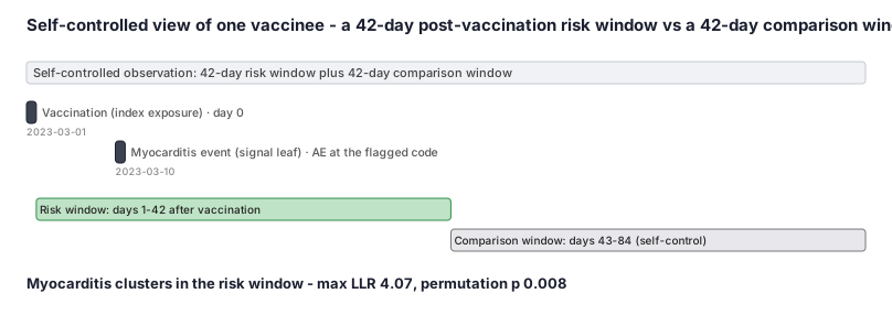
A new vaccine is monitored across a claims network. Events in the post-vaccination risk window are counted at four MedDRA Preferred Terms grouped under two System Organ Classes; expected counts come from the matched comparison person-time. The scan evaluates six cuts (four leaves + two branches), scores each with the conditional-Poisson LLR, takes the maximum, and benchmarks it against the permutation null. The worked_example below carries the exact, hand-checkable arithmetic - the myocarditis leaf wins with LLR 4.07 and a permutation p of about 0.017, nominating it as the candidate signal to confirm in a designed study.

Worked example

Scenario

A new vaccine is being watched in a claims network. In the weeks after vaccination we count adverse events at four specific MedDRA codes (the leaves), grouped under two broad categories (the branches): a cardiac category holding myocarditis and arrhythmia, and a GI category holding nausea and vomiting. From a matched comparison group we already know how many of each event we would expect if the vaccine were harmless. We want the scan to tell us which code, or which whole category, has a real excess - and to do it honestly even though we are checking six places at once.

Dataset

The counts an analyst feeds the scan - observed events in the vaccinated group and expected events from the matched comparison, for each leaf and each branch (a branch is just the sum of its leaves).

Steps

• Totals first - both columns sum to the same total because we conditioned on it. Observed = 8 + 2 + 3 + 2 = 15; expected = 3 + 3 + 5 + 4 = 15, so C = 15.

• The two branch cuts are just the sums of their leaves. Cardiac observed = 8 + 2 = 10, expected = 3 + 3 = 6. GI observed = 3 + 2 = 5, expected = 5 + 4 = 9.

• Only cuts with more events than expected can signal. Myocarditis (8 > 3) and cardiac (10 > 6) are in excess; arrhythmia, nausea, vomiting, and the whole GI branch all have fewer than expected, so their LLR is 0.

• Score the myocarditis leaf with the conditional-Poisson log-likelihood-ratio LLR = observed x ln(observed/expected) + (C - observed) x ln((C - observed)/(C - expected)). The observed-to-expected ratio there is 8 / 3 = 2.67, a clear excess.

• The excess term is 8 x ln(8/3), about 7.847, and the deficit term is 7 x ln(7/12), about -3.773, so the myocarditis LLR = 7.847 - 3.773 = 4.07.

• Score the cardiac branch the same way; its two terms are about 5.108 and -2.939, so its LLR = 5.108 - 2.939 = 2.17 - real, but smaller than the leaf, so the signal is the specific code, not the whole category.

• Take the maximum LLR over all six cuts (4.07 at myocarditis) as the test statistic, then shuffle - redistribute the 15 events across the four leaves in proportion to expected (3,3,5,4) hundreds of times and recompute the maximum each time. Suppose 7 of 999 shuffles produced a maximum LLR of at least 4.07.

• In 999 Monte Carlo permutations, 16 exceed the observed maximum, so the permutation p-value is (16 + 1) / (999 + 1) = 0.017 - the myocarditis cluster stands out across the whole tree after full multiplicity adjustment.

Result

The scan nominates the myocarditis leaf as the candidate signal (maximum LLR = 4.07, permutation p = 0.017); the cardiac branch is elevated (LLR 2.17) only because it contains myocarditis, and the GI side shows nothing. This is a hypothesis to confirm in a pre-specified, confounder-controlled study - not a confirmed harm.

Timeline Spec

Title

Self-controlled view of one vaccinee - a 42-day post-vaccination risk window vs a 42-day comparison window

Window

Start

2023-03-01

End

2023-05-24

Label

Self-controlled observation: 42-day risk window plus 42-day comparison window

Events

• Label

  Vaccination (index exposure)

  Start

  2023-03-01

  Length Days

  1

  Quantity

  day 0

• Label

  Myocarditis event (signal leaf)

  Start

  2023-03-10

  Length Days

  1

  Quantity

  AE at the flagged code

Spans

• Kind

  exposed

  Start

  2023-03-02

  End

  2023-04-12

  Label

  Risk window: days 1-42 after vaccination

• Kind

  unexposed

  Start

  2023-04-13

  End

  2023-05-24

  Label

  Comparison window: days 43-84 (self-control)

Result

Label

Myocarditis clusters in the risk window - max LLR 4.07, permutation p 0.017

Value

4.07

Runnable example

import math, random

LEAVES   = ["myocarditis", "arrhythmia", "nausea", "vomiting"]
OBSERVED = {"myocarditis": 8, "arrhythmia": 2, "nausea": 3, "vomiting": 2}   # sum = 15
EXPECTED = {"myocarditis": 3, "arrhythmia": 3, "nausea": 5, "vomiting": 4}   # conditioned to sum = 15
CUTS = {                                  # node -> leaves beneath it (leaf cuts + branch cuts)
    "myocarditis": ["myocarditis"],
    "arrhythmia":  ["arrhythmia"],
    "nausea":      ["nausea"],
    "vomiting":    ["vomiting"],
    "cardiac_SOC": ["myocarditis", "arrhythmia"],
    "gi_SOC":      ["nausea", "vomiting"],
}

def cut_llr(c, mu, C):
    # conditional-Poisson LLR for one cut; 0 unless the cut is in excess (c > mu)
    if c <= mu or c >= C:
        return 0.0
    return c * math.log(c / mu) + (C - c) * math.log((C - c) / (C - mu))

def scan(obs):
    C = sum(obs.values())
    best_node, best_llr = None, 0.0
    for node, members in CUTS.items():
        c  = sum(obs[m] for m in members)
        mu = sum(EXPECTED[m] for m in members)
        s  = cut_llr(c, mu, C)
        if s > best_llr:
            best_llr, best_node = s, node
    return best_llr, best_node

obs_llr, node = scan(OBSERVED)          # -> ~4.07 at "myocarditis"

C      = sum(OBSERVED.values())
weights = [EXPECTED[l] for l in LEAVES]
random.seed(20230601)
NSIM, hits = 999, 0
for _ in range(NSIM):
    draw = random.choices(LEAVES, weights=weights, k=C)   # redistribute C events under the null
    sim  = {l: 0 for l in LEAVES}
    for l in draw:
        sim[l] += 1
    if scan(sim)[0] >= obs_llr - 1e-9:
        hits += 1
p = (hits + 1) / (NSIM + 1)
print(f"most likely cut = {node}  LLR = {obs_llr:.2f}  permutation p = {p:.3f}")

leaves   <- c("myocarditis", "arrhythmia", "nausea", "vomiting")
observed <- c(myocarditis = 8, arrhythmia = 2, nausea = 3, vomiting = 2)   # sum = 15
expected <- c(myocarditis = 3, arrhythmia = 3, nausea = 5, vomiting = 4)   # conditioned to sum = 15
cuts <- list(myocarditis = "myocarditis", arrhythmia = "arrhythmia",
             nausea = "nausea", vomiting = "vomiting",
             cardiac_SOC = c("myocarditis", "arrhythmia"),
             gi_SOC      = c("nausea", "vomiting"))

cut_llr <- function(c, mu, C) {
  if (c <= mu || c >= C) return(0)
  c * log(c / mu) + (C - c) * log((C - c) / (C - mu))
}
scan <- function(obs) {
  C <- sum(obs); best_llr <- 0; best_node <- NA_character_
  for (node in names(cuts)) {
    m  <- cuts[[node]]
    s  <- cut_llr(sum(obs[m]), sum(expected[m]), C)
    if (s > best_llr) { best_llr <- s; best_node <- node }
  }
  list(llr = best_llr, node = best_node)
}
obs <- scan(observed)                       # -> ~4.07 at "myocarditis"

C       <- sum(observed)
weights <- expected[leaves] / sum(expected)
set.seed(20230601); NSIM <- 999L; hits <- 0L
for (i in seq_len(NSIM)) {
  draw <- sample(leaves, C, replace = TRUE, prob = weights)
  sim  <- setNames(as.integer(table(factor(draw, levels = leaves))), leaves)
  if (scan(sim)$llr >= obs$llr - 1e-9) hits <- hits + 1L
}
p <- (hits + 1L) / (NSIM + 1L)
cat(sprintf("most likely cut = %s  LLR = %.2f  permutation p = %.3f\n", obs$node, obs$llr, p))