Win Ratio and Generalized Pairwise Comparisons

In plain language

The win ratio compares a treatment group against a control group by pairing up patients and asking, for each pair, who did better on the most important outcome first - say, who lived longer - and only dropping to the next outcome (like who avoided a heart-failure hospitalization longer) if the first one is a tie. Across every treated-versus-control pair you count wins, losses, and ties, and the win ratio is simply wins divided by losses, so a number above 1 favors the treatment. Its big advantage over the usual "first event that happens" approach is that death can outrank a hospitalization instead of counting the same. Its big catch: if patients are followed for different lengths of time, many pairs become unrankable ties, which can pull the win ratio toward 1 and hide a real difference.

A composite endpoint stacks several outcomes into one. The classic real-world and trial answer is time-to-first-event: a patient counts the day the earliest of death, hospitalization, or any other listed event occurs, and a Cox model is run on that first event. This treats a heart-failure hospitalization on day 30 as equivalent to dying on day 30 - the model cannot tell which happened, because both are simply "the first event." That equivalence is clinically false and statistically wasteful: the most important outcome (death) is diluted by the most frequent one (hospitalization), and everything after the first event is thrown away.

The generalized pairwise comparison (GPC) idea

Instead of reducing each patient to a single first-event time, GPC compares every treated patient against every control patient as a pair. For each of the (n_treated x n_control) pairs you ask, in priority order: on the most important outcome, did the treated patient do better (a win), worse (a loss), or can we not tell (a tie)? If it is a tie on the top outcome, you drop to the next outcome in the hierarchy and ask again; you keep descending until the pair is separated or you run out of outcomes (an overall tie). Counting wins, losses, and ties across all pairs gives three related summaries: - Win ratio = wins / losses (ties excluded). A value above 1 favors treatment. - Win odds = (wins + 0.5 x ties) / (losses + 0.5 x ties). Ties are split evenly, so every pair contributes. - Net benefit (the Buyse statistic) = (wins - losses) / total pairs. A difference on the natural -1 to +1 scale.

The hierarchy is the analysis, and prioritization order is a real choice

You must pre-specify the ladder: death usually sits on top, then a serious morbidity event (HF hospitalization), then perhaps a continuous outcome (change in a biomarker or a quality-of-life score) for pairs still tied after the events. Reordering the ladder changes the estimate, because a different outcome gets first crack at separating each pair. Putting a frequent, less severe outcome on top makes the win ratio behave almost like time-to-first-event and forfeits the whole point; putting death on top lets mortality dominate, which is usually the intent. The order is a clinical judgment that belongs in the protocol, not a knob to tune after seeing results.

Matched vs unmatched comparisons

Pocock's original matched win ratio pairs each treated patient with a control of similar risk (matched on covariates or risk strata) and compares only within matched pairs. The unmatched / all-pairs version (Buyse's GPC, Finkelstein-Schoenfeld lineage) compares all treated-vs-control pairs and is the more common real-world form because it uses all the data and feeds directly into stratified and covariate-adjusted extensions. Both share the same win/loss/tie engine; they differ only in which pairs are formed.

Censoring is where win ratios get subtle

With time-to-event outcomes you often cannot order a pair: if a treated patient is censored (lost to follow-up, study ends) at day 200 and the control is still event-free at day 200, you do not know who would have had the event first - that pair is a tie on that tier by necessity, not because the patients are equivalent. Differential follow-up between arms can therefore manufacture ties and bias the win ratio toward 1, and the estimate depends on the follow-up time of the data (unlike a hazard ratio, which targets an instantaneous rate). Short or unequal follow-up inflates the tie count and can move the win ratio in either direction; this is the central caution for win ratios in real-world data, where follow-up is rarely uniform.

Interpreting the output

Consider a heart-failure registry study comparing a new device versus standard care on a two-tier hierarchy (Tier 1: cardiovascular death; Tier 2: HF hospitalization). Among all treated × control pairs, 1,540 pairs were won by the treated patient, 1,100 were lost, and 2,360 were tied. Win ratio = 1,540 / 1,100 = 1.40 (95% CI 1.15–1.71).

Formal interpretation: Among all treated–control patient pairs compared on the prioritized hierarchy, treated patients won on the more important outcome 1.40 times as often as they lost. A win is assigned by walking down the priority ladder: if the treated patient survived longer (Tier 1), that pair is a win regardless of HF events; only pairs tied on survival drop to Tier 2 (HF hospitalization). Ties remain when neither patient can be separated on any tier — typically because one or both were censored before the pair could be resolved. The win ratio of 1.40 is specific to this follow-up duration and censoring pattern; a study with shorter or more unequal follow-up would produce more ties and a win ratio closer to 1 for the same true effect.

Practical interpretation: Treated patients won on the priority hierarchy 40% more often than they lost. This framing deliberately lets death outweigh hospitalization — a patient who survives longer wins the pair even if they had more hospitalizations. Report the tie fraction (2,360 / (1,540 + 1,100 + 2,360) = 47%) alongside the win ratio because a high tie rate signals censoring-driven attenuation. The win ratio is not a hazard ratio and is not a per-unit-time rate; do not read 1.40 as "a 40% lower risk."

Pros, cons, and trade-offs

(specific and comparative). - vs composite-endpoint-construction-rwe (time-to-first-event): GPC's advantage is clinical weighting for free - death is allowed to outrank hospitalization without inventing arbitrary point values, and information after the first event is retained. Its costs are (a) dependence on follow-up time and censoring patterns, (b) a less familiar effect measure than a hazard ratio, and (c) sensitivity to the chosen hierarchy. Prefer GPC when the components differ sharply in severity and you want the worst outcome to dominate; prefer time-to-first-event when components are clinically comparable, follow-up is uniform, and a hazard ratio is the expected currency for the audience. - vs cox-ph-regression: A win ratio is not a hazard ratio and is not assumption-bound to proportional hazards - it can behave sensibly under non-proportional hazards and crossing curves where a single HR is misleading. But it sacrifices the hazard ratio's time-anchored interpretability, its established covariate-adjustment machinery, and its independence from total follow-up length. Prefer Cox when a per-unit-time rate is the target and PH roughly holds; prefer the win ratio when a prioritized composite and severity ranking matter more than a rate. - vs restricted-mean-survival-time-rmst: Both dodge the proportional-hazards assumption and both depend on a chosen time horizon, but RMST answers a single-endpoint question (mean event-free time up to tau) while GPC answers a hierarchical multi-endpoint question. Prefer RMST for one time-to-event outcome with a natural horizon; prefer GPC when several prioritized outcomes must be combined.

When to use

Hierarchical composite endpoints where components differ in severity and you want the most important to dominate - the canonical home is cardiology and heart-failure trials and their real-world emulations (cardiovascular death > HF hospitalization > symptom/biomarker change), and increasingly oncology (death > progression > response) and any setting with a clear clinical priority order. Use it when proportional hazards is doubtful, when a continuous outcome should break ties among event-free patients, or when stakeholders explicitly want mortality to outweigh softer endpoints rather than be averaged with them.

When NOT to use - and when it is actively misleading

- Severely unequal or short follow-up. If follow-up differs between arms (common in real-world cohorts with staggered entry and administrative censoring), uncomparable pairs become ties and the win ratio drifts toward 1, masking a true effect; align follow-up, restrict to a common horizon, or use a method robust to dependent censoring before trusting the number. Do not report a win ratio from data with grossly differential censoring without that caution. - No genuine priority order. If the components are clinically interchangeable (two equally serious events with no agreed ranking), forcing a hierarchy invents an ordering that drives the result; a time-to-first-event or recurrent-event analysis is more honest. - Reading the win ratio as a hazard ratio or a rate. It is a ratio of wins to losses over a specific follow-up window, not a per-time hazard; quoting "a 30% lower risk" from a win ratio of 1.43 is wrong. Report it as what it is, with the follow-up horizon and the tie fraction, because both are part of the estimand. - Confounding is unaddressed by the engine. All-pairs comparison does not adjust for confounding any more than a crude rate does; in observational data you still need matching, stratification, or weighting (e.g., on a propensity score) layered onto the pair formation, or the win ratio just compares confounded groups efficiently.

Worked example

Scenario

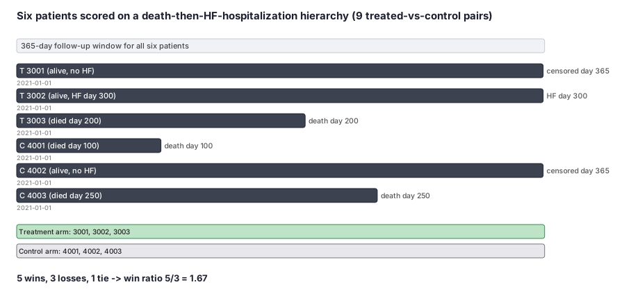
A heart-failure treatment is compared against control using a two-level priority: first survival (did the patient live longer), then time to the first heart-failure hospitalization for pairs that tie on survival. We have three treated and three control patients, each followed up to 365 days. We compare all 3 x 3 = 9 treated-versus-control pairs, label each a win, loss, or tie for the treatment, and compute the win ratio, win odds, and net benefit by hand.

Dataset

One row per patient. death_day and hf_hosp_day are 'none' if the event was not observed; followup_day is the last day the patient was seen.

Steps

• Tier 1 rule (survival), longer life wins. Tier 2 rule (used only if Tier 1 ties), longer time to first HF hospitalization wins. A pair is a tie if neither tier can separate the two patients.

• Treated 3001 (alive, no HF) vs each control. vs 4001 (died day 100), vs 4003 (died day 250), it outlives them so 3001 WINS both; vs 4002 (also alive, no HF) nothing separates them so TIE. That is 2 wins and 1 tie.

• Treated 3002 (alive, HF day 300) vs controls. vs 4001 and vs 4003 it outlives both (WIN, WIN); vs 4002 both survive so Tier 1 ties, then Tier 2 compares HF - 3002 was hospitalized on day 300 but 4002 stayed event-free past day 300, so 4002 wins and 3002 LOSES. That is 2 wins and 1 loss.

• Treated 3003 (died day 200) vs controls. vs 4001 (died day 100) it survived longer so WIN; vs 4002 (alive at 365) and vs 4003 (died day 250) the controls outlive it, so 3003 LOSES both. That is 1 win and 2 losses.

• Totals across the 9 pairs - wins = 2 + 2 + 1 = 5, losses = 0 + 1 + 2 = 3, ties = 1 + 0 + 0 = 1.

• Win ratio = wins / losses = 5 / 3 = 1.67. Net benefit = (5 - 3) / 9 = 0.22. Win odds (split the tie) = (5 + 0.5) / (3 + 0.5) = 1.57.

Result

Across 9 pairs there are 5 wins, 3 losses, and 1 tie, so the win ratio = 5 / 3 = 1.67 (favoring treatment), the win odds = (5 + 0.5) / (3 + 0.5) = 1.57, and the net benefit = (5 - 3) / 9 = 0.22. Survival decided most pairs; HF hospitalization only broke the single Tier-1 tie between 3002 and 4002.

Timeline Spec

Title

Six patients scored on a death-then-HF-hospitalization hierarchy (9 treated-vs-control pairs)

Window

Start

2021-01-01

End

2022-01-01

Label

365-day follow-up window for all six patients

Events

• Label

  T 3001 (alive, no HF)

  Start

  2021-01-01

  Length Days

  365

  Quantity

  censored day 365

• Label

  T 3002 (alive, HF day 300)

  Start

  2021-01-01

  Length Days

  365

  Quantity

  HF day 300

• Label

  T 3003 (died day 200)

  Start

  2021-01-01

  Length Days

  200

  Quantity

  death day 200

• Label

  C 4001 (died day 100)

  Start

  2021-01-01

  Length Days

  100

  Quantity

  death day 100

• Label

  C 4002 (alive, no HF)

  Start

  2021-01-01

  Length Days

  365

  Quantity

  censored day 365

• Label

  C 4003 (died day 250)

  Start

  2021-01-01

  Length Days

  250

  Quantity

  death day 250

Spans

• Kind

  exposed

  Start

  2021-01-01

  End

  2022-01-01

  Label

  Treatment arm: 3001, 3002, 3003

• Kind

  unexposed

  Start

  2021-01-01

  End

  2022-01-01

  Label

  Control arm: 4001, 4002, 4003

Result

Label

5 wins, 3 losses, 1 tie -> win ratio 5/3 = 1.67

Value

1.67

Runnable example

from math import inf

def _surv(p):
    # death time if it happened, else +inf; censoring (last observed) time
    return (p["death_day"] if p["death_day"] is not None else inf,
            p["followup_day"])

def _hf(p):
    return (p["hf_day"] if p["hf_day"] is not None else inf,
            p["followup_day"])

def compare_pair(t, c):
    # returns +1 = treated wins, -1 = treated loses, 0 = tie (descend / overall tie)
    # Tier 1: longer survival wins; indeterminate under censoring -> descend
    td, tcens = _surv(t); cd, ccens = _surv(c)
    if td != inf and cd != inf:
        if td > cd: return 1
        if td < cd: return -1
    elif td != inf and cd == inf:          # treated died, control censored
        if ccens >= td: return -1           # control known to outlive treated's death
    elif cd != inf and td == inf:          # control died, treated censored
        if tcens >= cd: return 1
    # Tier 2: longer time to first HF hospitalization wins
    th, thc = _hf(t); ch, chc = _hf(c)
    if th != inf and ch != inf:
        if th > ch: return 1
        if th < ch: return -1
    elif th != inf and ch == inf:          # treated had HF, control event-free
        if chc >= th: return -1
    elif ch != inf and th == inf:          # control had HF, treated event-free
        if thc >= ch: return 1
    return 0

def win_ratio(subjects):
    tx = [s for s in subjects if s["arm"] == "treatment"]
    ct = [s for s in subjects if s["arm"] == "control"]
    wins = losses = ties = 0
    for t in tx:
        for c in ct:
            r = compare_pair(t, c)
            if r == 1: wins += 1
            elif r == -1: losses += 1
            else: ties += 1
    total = wins + losses + ties
    return {
        "wins": wins, "losses": losses, "ties": ties, "pairs": total,
        "win_ratio": wins / losses if losses else inf,
        "win_odds": (wins + 0.5 * ties) / (losses + 0.5 * ties) if (losses + 0.5 * ties) else inf,
        "net_benefit": (wins - losses) / total if total else 0.0,
    }

compare_pair <- function(t, c) {
  td <- if (is.na(t$death_day)) Inf else t$death_day; tcens <- t$followup_day
  cd <- if (is.na(c$death_day)) Inf else c$death_day; ccens <- c$followup_day
  # Tier 1: survival
  if (is.finite(td) && is.finite(cd)) {
    if (td > cd) return(1L); if (td < cd) return(-1L)
  } else if (is.finite(td) && is.infinite(cd)) {
    if (ccens >= td) return(-1L)
  } else if (is.finite(cd) && is.infinite(td)) {
    if (tcens >= cd) return(1L)
  }
  # Tier 2: time to first HF hospitalization
  th <- if (is.na(t$hf_day)) Inf else t$hf_day
  ch <- if (is.na(c$hf_day)) Inf else c$hf_day
  if (is.finite(th) && is.finite(ch)) {
    if (th > ch) return(1L); if (th < ch) return(-1L)
  } else if (is.finite(th) && is.infinite(ch)) {
    if (c$followup_day >= th) return(-1L)
  } else if (is.finite(ch) && is.infinite(th)) {
    if (t$followup_day >= ch) return(1L)
  }
  0L
}

win_ratio <- function(df) {
  tx <- df[df$arm == "treatment", ]; ct <- df[df$arm == "control", ]
  wins <- 0L; losses <- 0L; ties <- 0L
  for (i in seq_len(nrow(tx))) for (j in seq_len(nrow(ct))) {
    r <- compare_pair(as.list(tx[i, ]), as.list(ct[j, ]))
    if (r == 1L) wins <- wins + 1L
    else if (r == -1L) losses <- losses + 1L
    else ties <- ties + 1L
  }
  total <- wins + losses + ties
  list(wins = wins, losses = losses, ties = ties, pairs = total,
       win_ratio = if (losses > 0) wins / losses else Inf,
       win_odds  = (wins + 0.5 * ties) / (losses + 0.5 * ties),
       net_benefit = (wins - losses) / total)
}