Case-Cohort Design

In plain language

A case-cohort study starts with a large group of patients all followed over time, then picks a smaller random sample — the subcohort — at the very beginning, before anyone develops the outcome of interest. Researchers only run expensive tests (like biomarker blood assays or detailed chart reviews) on subcohort members plus any patients who later develop the outcome, instead of testing everyone. The big advantage over a similar approach called nested case-control is that the same subcohort can be reused for several different outcomes, and you can also calculate how common the outcome was in the whole group — not just compare those who got it to those who did not. However, the statistical analysis requires a special weighted version of the Cox survival model; using the standard unweighted version on this kind of data is a known mistake that produces incorrect results.

Design mechanics

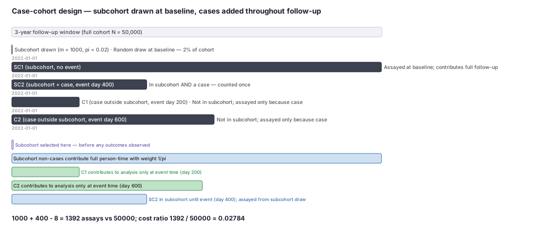
The case-cohort design begins, like all nested sampling designs, with a fully assembled and enrolled cohort — every member has a time-zero, an eligibility record, and an observable follow-up period. At baseline (time-zero), before any outcomes are observed, the analyst draws a random subcohort of size m from the full cohort of size N, yielding a sampling fraction π = m / N. During follow-up, the study team ascertains expensive covariates — stored biospecimen assays, manual chart abstraction, genotyping, imaging reads — for every subcohort member, regardless of whether they later develop the outcome. As cases accumulate anywhere in the full cohort, any case not already in the subcohort is added to the measurement queue; the covariate is ascertained for them as well. The analytic dataset therefore contains: (1) all subcohort members (cases and non-cases alike), and (2) cases from outside the subcohort. The key quantity is the overlap: cases who happen to fall inside the subcohort by chance are counted once, not twice. Total assays = m + (total cases) − (cases inside subcohort).

The killer advantage over nested case-control: one subcohort, many outcomes

In a nested case-control (NCC) design, controls are sampled fresh at each case's event time and are therefore outcome-specific — a new control sample is needed for every endpoint. The case-cohort subcohort is drawn once at baseline and reused for every outcome the study examines: fatal myocardial infarction, incident diabetes, all-cause mortality, and any post-hoc endpoint can each use the same m subcohort members, with only the new-case set varying. This makes case-cohort the preferred design for multi-endpoint biobank and registry substudies.

Absolute risk is estimable

Because the subcohort is a probability sample of the full cohort, its person-time is a known fraction of the total cohort person-time, and event rates (incidence densities) and cumulative incidence can be estimated with appropriate weighting. NCC, by contrast, cannot recover absolute risks without additional data because the risk-set sampling probabilities depend on cohort size in a time-varying way that is not always recorded.

Pros, cons, and trade-offs

• vs full-cohort Cox: The case-cohort design's sole advantage is measurement cost when an

• vs nested case-control: NCC re-samples controls at each event time, providing tight

• vs self-controlled designs (SCCS, case-crossover): Self-controlled designs eliminate

The classic analytic mistake: unweighted Cox

Because the subcohort is a biased sample of the risk sets at later event times (subcohort members who died or were censored early are underrepresented in later risk sets), naive Cox regression on the case-cohort dataset without weights produces a biased hazard-ratio estimate. The correct analysis uses a weighted pseudo-partial likelihood in which the contribution of each subcohort non-case at each event time is up-weighted by 1/π to represent the full cohort's at-risk pool. Two main weighting schemes exist: Prentice (1986) weights, which use 1/π for subcohort members who have not yet failed and 1 for cases at their event time; and Barlow et al. (1999) weights (also called self-weighted or "Barlow"), which assign a constant weight of 1/π to subcohort members throughout follow-up and 1 to all cases at their event time, yielding slightly simpler implementation and the same asymptotic estimator. Both require a robust (sandwich) variance estimator because the same subcohort members appear in multiple pseudo-risk sets and the standard Cox variance ignores this correlation. The `survival::cch` function in R implements both methods and the robust variance directly.

When to use

A retrospective cohort with expensive covariates (biospecimen assays, manual chart abstraction, genotyping, expert adjudication) that cannot be collected cost-effectively for all N members; multi-outcome or multi-endpoint biobank or registry substudies where one sampled panel is to serve several hypotheses; situations where absolute incidence rates or cumulative incidence are needed alongside relative risks; and claims or EHR cohorts being linked to chart-validated outcome data for a validation substudy, where the chart-pull is the expensive item.

When NOT to use — and when it is actively misleading or dangerous

• Cheap, complete exposure in claims/EHR. If the covariate of interest is already coded
• Unweighted Cox on the case-cohort dataset. Fitting a standard (unweighted) Cox model
• Highly time-varying expensive exposure. If the expensive item is a time-varying
• Very small cohorts. With N < several hundred, the subcohort may be nearly the full
• Ignoring overlap between cases and subcohort. Double-counting cases who are also

Interpreting the output

The weighted Cox estimator from a correctly analyzed case-cohort produces a hazard-ratio coefficient for each covariate. Using the worked example: cohort N = 50,000, subcohort m = 1,000 (π = 0.02), 400 total cases, 8 inside the subcohort; suppose the Barlow-weighted analysis yields HR = 1.73 (robust 95% CI 1.31–2.28) for the exposure of interest.

Formal interpretation: The Barlow-weighted Cox partial-likelihood estimator, with robust sandwich variance to account for the repeated appearance of subcohort members across pseudo-risk sets, estimates an instantaneous rate ratio of 1.73 comparing exposed to unexposed subjects among those still at risk at each event time. The confidence interval has the repeated-sampling interpretation: if this analysis were repeated many times under the same sampling design, approximately 95% of such intervals would contain the true hazard ratio in the source cohort. The estimate is conditional on measured covariates and requires the untestable assumption that unmeasured confounders are not materially associated with both exposure and outcome.

Practical interpretation: At any moment during follow-up, exposed patients had approximately 73% higher instantaneous risk of the outcome than unexposed patients of the same measured characteristics. The confidence interval (1.31 to 2.28) excludes 1.0, indicating this association is unlikely to be due to chance, though residual unmeasured confounding cannot be ruled out in an observational study.

Data-source operational depth

• Claims with chart-validated outcomes: The classic RWE application is a large claims
• Registry biomarker substudies: A disease registry fixes the case set (all diagnoses are
• EHR cohorts: Define the cohort from encounter-based enrollment windows; the subcohort is
• Competing risks: In elderly or seriously ill cohorts, death may compete with the primary

Worked example

Scenario

A research team assembles a cohort of 50,000 adults from a linked claims-registry database to study whether a costly biomarker measured from stored serum predicts incident cardiovascular events. Running the assay on all 50,000 patients would cost roughly $500 per assay. Instead, they draw a subcohort of 1,000 patients at random at baseline (day zero), before any events occur. Over three years of follow-up, 400 patients across the full cohort develop the outcome; of those 400 cases, 8 were already in the subcohort. The team needs to calculate exactly how many assays are required and compare that to the full-cohort alternative.

Dataset

Summary counts for the case-cohort calculation — not one row per patient but the key group totals an analyst would record before deciding on the design.

Steps

• Sampling fraction: subcohort size divided by full cohort size gives 1000 / 50000 = 0.02, meaning 2% of the cohort is in the subcohort.

• Cases outside the subcohort: 400 total cases minus the 8 who were already selected into the subcohort gives 400 - 8 = 392 additional subjects needing an assay.

• Total assays required: all subcohort members plus all cases not already in the subcohort gives 1000 + 392 = 1392 assays.

• Cross-check using the overlap formula: subcohort size plus all cases minus cases inside the subcohort gives 1000 + 400 - 8 = 1392 assays — confirming the same answer.

• Cost ratio versus full-cohort measurement: 1392 / 50000 = 0.02784, meaning only about 2.8% as many assays are needed compared to measuring everyone.

• Because the subcohort is a probability sample drawn at baseline, it can be reused for a second or third outcome (say, incident diabetes or all-cause mortality) without any additional assays on the subcohort members — only new cases outside the subcohort for each additional outcome would require measurement, making the multi-outcome cost savings even larger.

Result

Total assays = 1000 + 400 - 8 = 1392 versus 50000 for full-cohort measurement. Cost ratio 1392 / 50000 = 0.02784 (approximately 2.8% of the full-cohort burden). The subcohort is then reused for every additional outcome at no extra baseline cost.

Timeline Spec

Title

Case-cohort design — subcohort drawn at baseline, cases added throughout follow-up

Window

Start

2022-01-01

End

2025-01-01

Label

3-year follow-up window (full cohort N = 50,000)

Events

• Label

  Subcohort drawn (m = 1000, pi = 0.02)

  Start

  2022-01-01

  Length Days

  1

  Quantity

  Random draw at baseline — 2% of cohort

• Label

  SC1 (subcohort, no event)

  Start

  2022-01-01

  Length Days

  1096

  Quantity

  Assayed at baseline; contributes full follow-up

• Label

  SC2 (subcohort + case, event day 400)

  Start

  2022-01-01

  Length Days

  400

  Quantity

  In subcohort AND a case — counted once

• Label

  C1 (case outside subcohort, event day 200)

  Start

  2022-01-01

  Length Days

  200

  Quantity

  Not in subcohort; assayed only because case

• Label

  C2 (case outside subcohort, event day 600)

  Start

  2022-01-01

  Length Days

  600

  Quantity

  Not in subcohort; assayed only because case

Spans

• Kind

  washout

  Start

  2022-01-01

  End

  2022-01-01

  Label

  Subcohort selected here — before any outcomes observed

• Kind

  followup

  Start

  2022-01-01

  End

  2024-12-31

  Label

  Subcohort non-cases contribute full person-time with weight 1/pi

• Kind

  exposed

  Start

  2022-01-01

  End

  2022-07-19

  Label

  C1 contributes to analysis only at event time (day 200)

• Kind

  exposed

  Start

  2022-01-01

  End

  2023-07-19

  Label

  C2 contributes to analysis only at event time (day 600)

• Kind

  followup

  Start

  2022-01-01

  End

  2023-02-04

  Label

  SC2 in subcohort until event (day 400); assayed from subcohort draw

Result

Label

1000 + 400 - 8 = 1392 assays vs 50000; cost ratio 1392 / 50000 = 0.02784

Value

0.02784

Caption

Subcohort members (SC1, SC2) contribute follow-up time throughout the study with up-weights of 1/pi = 50 representing the full cohort risk pool. Cases outside the subcohort (C1, C2) are added to the analytic dataset only because they are cases; they receive weight 1 at their event time. SC2, who is both a subcohort member and a case, is counted once with the case weight at their event time. The single subcohort can be reused for additional outcomes without re-drawing.

Alt Text

Timeline showing three years of follow-up from 2022 to 2025. A marker at the 2022-01-01 baseline shows the subcohort drawn from the full cohort. Subcohort member SC1 has a full-length follow-up bar. SC2's bar ends at day 400 with a case marker. Two additional case bars (C1 at day 200, C2 at day 600) are shorter and labeled as cases outside the subcohort. A note indicates 1392 total assays versus 50000 for the full cohort.

Runnable example

import pandas as pd
from lifelines import CoxPHFitter

def build_case_cohort_weights(cohort: pd.DataFrame, pi: float) -> pd.DataFrame:
    """
    Assign Barlow weights to the case-cohort analytic dataset.

    Barlow rule:
      - All subcohort members (cases + non-cases): weight = 1 / pi during
        their non-event follow-up.
      - All cases (in subcohort or not): weight = 1 at their event time.
    For a counting-process approximation in lifelines, we use a single-row
    per subject and set weight = 1 for cases, 1/pi for subcohort non-cases.
    Subcohort members who are also cases receive weight = 1 (case dominates).

    This is a Barlow approximation; use survival::cch in R for the exact estimator.
    """
    df = cohort.copy()

    # Only include subjects in the analytic dataset:
    #   - all subcohort members
    #   - all cases (whether in subcohort or not)
    analytic = df[df["in_subcohort"] | (df["event"] == 1)].copy()

    # Barlow weight: 1 for cases, 1/pi for subcohort non-cases.
    analytic["weight"] = analytic.apply(
        lambda r: 1.0 if r["event"] == 1 else 1.0 / pi, axis=1
    )

    return analytic

# --- example usage ---
# cohort  = pd.DataFrame(...)  # one row per subject, biomarker ascertained for subcohort + cases
# N = len(cohort)              # full cohort size
# m = cohort["in_subcohort"].sum()
# pi = m / N                   # sampling fraction

pi = 0.02   # 1000 / 50000 in the worked example

# Build the analytic dataset.
analytic = build_case_cohort_weights(cohort, pi)

# Compute follow-up duration in days.
analytic["duration"] = (
    pd.to_datetime(analytic["exit_date"]) - pd.to_datetime(analytic["entry_date"])
).dt.days

# Fit Barlow-weighted Cox with robust variance.
cph = CoxPHFitter()
cph.fit(
    analytic[["duration", "event", "biomarker", "weight"]],
    duration_col="duration",
    event_col="event",
    weights_col="weight",
    robust=True   # sandwich variance — required for case-cohort; corrects for
                  # repeated subcohort membership across pseudo-risk sets
)
cph.print_summary()
# exp(coef) for biomarker is the Barlow-weighted hazard ratio.
# For publishable analyses use R survival::cch or SAS PROC PHREG with COVS(AGGREGATE).

library(survival)

# --- worked example parameters ---
N  <- 50000L   # full cohort size
m  <- 1000L    # subcohort size  (drawn at baseline)
pi <- m / N    # sampling fraction: 1000 / 50000 = 0.02

# dat: analytic dataset — subcohort members + all cases.
# Build in advance; biomarker is NA for non-subcohort non-cases (they are excluded).
# One row per subject; in_subcohort = TRUE/FALSE; event = 0/1.

# Barlow method (recommended for most applied settings):
fit_barlow <- cch(
  Surv(entry, exit, event) ~ biomarker + exposure,
  data        = dat,
  subcoh      = ~in_subcohort,       # logical column marking subcohort membership
  id          = ~person_id,
  cohort.size = N,                   # full cohort N — required for weight computation
  method      = "Barlow"             # alternatives: "Prentice", "II.Borgan"
)
summary(fit_barlow)
# exp(coef) is the Barlow-weighted hazard ratio with robust 95% CI.
# The robust variance (sandwich) is applied automatically by cch().

# Prentice method for comparison:
fit_prentice <- cch(
  Surv(entry, exit, event) ~ biomarker + exposure,
  data        = dat,
  subcoh      = ~in_subcohort,
  id          = ~person_id,
  cohort.size = N,
  method      = "Prentice"
)
summary(fit_prentice)

# Both should produce similar HR estimates; CIs will differ slightly.
# In the worked example (pi = 0.02, 400 cases, 8 in subcohort):
# assays required = 1000 + 400 - 8 = 1392 vs 50000 full-cohort.