The Hazard Ratio as an Effect Measure

In plain language

A hazard ratio (HR) compares how quickly an event — like a death, hospitalization, or disease progression — arrives in one treatment group versus another at each moment that both groups still have patients who have not yet had the event. An HR of 2.0 means the exposed group has events arriving at twice the speed of the comparison group at any given instant; it is NOT the same as saying there are twice as many events overall or that patients face twice the lifetime risk. Because the HR is calculated only among those still event-free at each moment, its meaning can shift over time as the riskiest patients leave the study first, making a single number potentially misleading for long follow-up. Always pair the HR with an absolute measure — such as the difference in average event-free months or the difference in event probability at a specific time point — so that decision-makers can judge whether the relative improvement translates to a meaningful real-world benefit.

The hazard as an instantaneous rate

The hazard at time t — written h(t) — is the probability that an event occurs at exactly the instant t, given that the subject has survived to t, expressed as a rate per unit time. Formally h(t) = lim_{Δt→0} P(t ≤ T < t+Δt | T ≥ t) / Δt. It is not a probability bounded between 0 and 1; it is a rate, and it is defined only among individuals who are still event-free at that moment. The hazard ratio HR = h_A(t) / h_B(t) compares these instantaneous rates between two groups. Under the proportional hazards (PH) assumption — that this ratio is constant across all t — Cox regression summarizes the entire follow-up as a single dimensionless number. When PH fails, the Cox partial likelihood produces a weighted average of time-varying, period-specific HRs, with weights that depend on the censoring distribution and on the size of the risk set at each event time. The resulting single-number summary then depends on study duration and dropout pattern, not just the underlying biology.

Hazard ≠ risk: the measure that matters for decisions

Risk is a cumulative probability — the chance the event occurs by a stated time horizon. Hazard is an instantaneous rate among survivors. They are linked through the survival function S(t) = exp(−∫₀ᵗ h(u) du), and cumulative incidence (risk) equals 1 − S(t). Under constant hazard and rare events over short windows, HR approximates the risk ratio (RR). For common events or long follow-up they can diverge substantially. The HR also differs from the aggregate rate ratio in the person-time sense, which is (events_A / person-time_A) ÷ (events_B / person-time_B); that equals the HR only when hazard is constant within each arm throughout follow-up. The practical implication: the HR cannot be inserted into a Markov state-transition model, a budget-impact calculation, or a cost-per-QALY denominator without first converting it to an absolute survival curve via the Breslow baseline estimator. Always report the RMST difference, landmark cumulative incidence difference, or median survival difference alongside the HR.

The Hernán critique: depletion of susceptibles and estimand ambiguity

Hernán (2010) in "The Hazards of Hazard Ratios" articulated the most important conceptual trap in survival analysis: even in a perfectly randomized trial — no confounding, no informative censoring — a single reported HR is causally ambiguous when the proportional hazards assumption does not hold. The mechanism is depletion of susceptibles. Individuals most vulnerable to the event fail early, and disproportionately so in the higher-hazard arm. As time passes, the surviving risk sets in both arms become self-selected, and the two groups are no longer exchangeable even under perfect randomization. A genuine constant treatment effect can therefore produce an observed HR that drifts over follow-up as the composition of the risk sets changes. Immuno-oncology provides the canonical example: checkpoint inhibitors often produce a delayed Kaplan-Meier curve separation — no early benefit, then strong late benefit. A single averaged HR from a log-rank test or Cox model blends the null early period with the effective late period, and the weights on each period vary by how long patients were followed and how many were censored. A study with more late follow-up produces a numerically different HR for the same biology than an otherwise identical study with shorter follow-up. This is Hernán's central point: the HR is partly a function of study design, not just the causal effect. Stensrud and Hernán (2020) extend this to argue that the right question is not "does PH hold?" but "what is the estimand I actually want?" — cumulative incidence difference at year 2? Mean event-free months over 3 years? — and to pre-specify it before data analysis begins, reporting the HR only as a supplementary relative summary alongside an absolute measure that is invariant to censoring patterns.

Noncollapsibility of the hazard ratio

The HR shares with the odds ratio the property of noncollapsibility: even when a covariate is not a confounder — it is balanced between arms and affects only the outcome — adjusting for it changes the HR. The conditional (adjusted) HR is generally farther from the null than the marginal (unadjusted) HR when the covariate is prognostic; this direction holds under most standard hazard structures but is not algebraically guaranteed for all combinations of hazard shape and covariate distribution. Three practical implications follow. (1) A covariate-adjusted Cox HR is typically larger in magnitude than the log-rank HR from an unadjusted Kaplan-Meier analysis — this is not evidence of confounding, it is the arithmetic consequence of noncollapsibility. (2) An HR from a propensity-score-matched or IPTW-weighted analysis estimates a marginal quantity, while the Cox HR is conditional on the covariate pattern in the model; they answer different questions and should not be compared across papers without acknowledging this distinction. (3) In an RCT, adding a strong prognostic baseline covariate to the Cox model will move the HR for treatment even when the covariate is perfectly balanced — this is expected and represents an efficiency gain, not an indication of imbalance or error.

Interpreting the output

Consider a study reporting HR = 0.75 (95% CI 0.60–0.94) for a new treatment versus standard care, from a Cox model with baseline covariate adjustment.

Formal interpretation: At any given instant during follow-up, among patients who have not yet had the event, the instantaneous rate of the event is 25% lower in the treated group than in the comparator group. This is NOT a statement that there are 25% fewer events in total. It is NOT a risk ratio, which compares cumulative probabilities of the event by a fixed horizon. It is NOT a time ratio, which would say the treated arm takes 1/0.75 = 1.33 times longer on average to reach the event. Under PH the 0.75 is a valid summary across all time points. Under non-PH it is a weighted average of period-specific HRs, where the weights depend on the censoring distribution — making the number partly an artifact of study duration and dropout pattern. Additionally, the built-in depletion of susceptibles means that even under PH the late-period HR reflects a causally different risk-set composition than the early-period HR. The 95% CI of 0.60–0.94 is a repeated- sampling interval: under the same data-generating process, approximately 95% of intervals constructed this way would contain the true HR. This CI excludes 1.0, but it is not a p-value statement about the probability of an extreme result under the null hypothesis.

Practical interpretation: Treated patients experience events at a 25% slower rate while they remain event-free. Paired with an absolute summary for this study's 2-year follow-up: the RMST difference was 2.8 months (treated patients gained 2.8 additional event-free months on average), and the risk difference at 24 months was approximately 6 fewer events per 100 patients in the treated arm. A payer or HTA reviewer cannot act on "HR 0.75" alone — the absolute benefit determines whether the treatment is cost-effective. Always pair the HR with the RMST difference, landmark risk difference, or median survival difference. This absolute-measure pairing is not optional: it is required by NICE, EMA guidelines for survival extrapolation, and the FDA's 2023 guidance on estimands in clinical trials.

RWE-specific interpretation challenges

Two issues in observational data compound the standard warnings. First, informative censoring: when patients disenroll from the health plan before the event for reasons related to their prognosis, they are administratively removed from the risk set. The direction of bias depends on which arm experiences more prognosis-related censoring and on the true direction of the treatment effect. For example, if sicker treated patients disenroll due to adverse effects, their removal inflates apparent survival in the treated arm and biases the HR away from the null (toward apparent benefit). Conversely, if sicker untreated patients disenroll first, the HR can be biased toward the null. There is no universally safe direction to assume; the bias must be assessed case by case. Inverse probability of censoring weighting (IPCW) corrects this by upweighting remaining patients for those who were censored due to prognosis-related reasons; the resulting HR corresponds to the counterfactual world where all patients remained observable. Second, time-varying exposures: the HR from a time-fixed baseline-exposure Cox model reflects initial treatment assignment, not sustained treatment. When patients switch, discontinue, or titrate their regimen, a counting-process layout (start, stop, event intervals) with exposure updated at each interval is required for an as-treated or per-protocol analysis. Naive time-fixed analysis in the presence of switching produces an HR that blends on-treatment and off-treatment periods — estimand-ambiguous for the same reason as Hernán's depletion-of-susceptibles argument. For the related trap of inflated exposed person-time from misaligned time zero, see immortal-time-bias-handling.

Pros, cons, and trade-offs

Pros of the HR as an effect measure: compact and dimensionless; directly estimated by Cox regression with adjustment for baseline covariates and time-varying factors; the standard language of survival analysis familiar to FDA, EMA, and clinical journal reviewers; efficient when PH holds; can be stratified, time-segmented, or marginalized via IPTW to handle specific violations; has mature, validated software across all three major analytic languages.

Cons: Non-collapsible — conditional and marginal HRs are not comparable across studies with different covariate profiles. Estimand-ambiguous under non-PH — the value depends on censoring distribution and study duration, not just the causal effect. Not directly interpretable as a probability or risk. Cannot be used in decision models without converting to survival curves. The depletion-of-susceptibles mechanism makes the single HR causally murky in long follow-up studies, particularly in oncology. A large relative improvement (HR = 0.50) in a very rare event may translate to trivially small absolute benefit; the HR alone conceals this.

Trade-offs vs. RMST difference: RMST requires no PH assumption, is absolute (event-free months gained), and is directly interpretable by patients, payers, and HTA bodies. Cost: lower power than log-rank and Cox under PH; requires pre-specifying the horizon; less familiar to some regulatory reviewers. Best practice is to pre-specify both and report both. Trade-offs vs. landmark risk difference or risk ratio at a fixed time: risk at a pre-specified landmark is a direct probability, natural for patient communication, budget- impact models, and Markov model inputs. Cost: discards information about when during follow-up events occur; sensitive to landmark choice.

When to use

Use the HR — always paired with an absolute summary — when: (a) Cox regression is the pre-specified analytic method for a time-to-event endpoint with a defensible time zero; (b) the audience expects a relative effect on the hazard scale, as in regulatory submissions and pharmacoepidemiology journals; (c) proportional hazards approximately holds (Kaplan-Meier curves are roughly parallel, Schoenfeld residual test is non- significant for the treatment variable); and (d) a companion absolute measure — RMST difference, cumulative incidence difference at a landmark, or median survival difference — is pre-specified and reported alongside it. The HR remains a valid descriptive summary under mild PH violations, interpreted as a weighted average of period-specific rates rather than a period-invariant constant.

When NOT to use

Do not use the HR as the sole effect measure when: (a) hazards cross or converge — a non-PH violation visible on a log-log survival plot or flagged by a significant Schoenfeld test means the single averaged HR is actively misleading; report RMST difference or time- segmented HRs instead; (b) the audience is patients or non-specialist clinicians who will interpret it as a percentage of events or a probability — it is neither; (c) the result feeds directly into an HTA cost-effectiveness model requiring transition probabilities or state-occupancy times — convert to survival curves and absolute risks first; (d) competing risks are substantial and differential by arm, as in elderly or end-stage populations — the cause-specific HR from Cox overstates absolute incidence of the event of interest and must be paired with a subdistribution HR and cumulative incidence function; (e) the study uses time-varying exposures without a counting-process layout — the resulting number is a blend of on- and off-treatment periods with no clear causal interpretation.

Worked example

Scenario

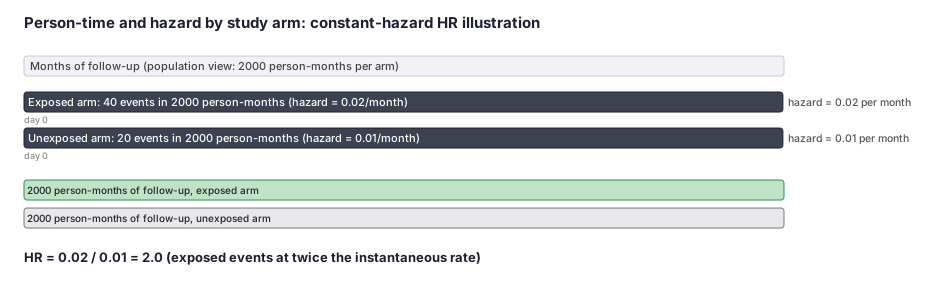
A researcher compares two groups — a new drug (exposed) versus standard care (unexposed) — in a registry study tracking time to a composite cardiovascular event. Aggregate person-time data are available for each arm. Under a constant-hazard assumption (rates are stable over follow-up), the hazard ratio can be computed directly from the event rates, illustrating exactly what the HR means and why it is not a risk ratio. Median event-free time under constant hazard is shown descriptively to illustrate how the HR relates to the time-ratio measure used in accelerated failure time models.

Dataset

Group-level person-time summary for two study arms under a constant-hazard assumption. Each row is one treatment arm. Person-months is the total follow-up accumulated by all patients in that arm; hazard_per_pm is the event rate per person-month.

Steps

• Compute the exposed hazard rate: 40 / 2000 = 0.02 events per person-month. This means that at any given month, among those still event-free, the new-drug arm has an event rate of 0.02 per person-month.

• Compute the unexposed hazard rate: 20 / 2000 = 0.01 events per person-month.

• Compute the hazard ratio (exposed vs. unexposed): 0.02 / 0.01 = 2.0. The exposed group has events at twice the instantaneous rate of the unexposed group at any given moment, among those still event-free at that moment.

• Interpretation check — this is NOT a risk ratio: the HR of 2.0 does not mean twice as many events will occur overall. Risk over a finite window depends on the hazard AND the length of the window. For 12 months under constant hazard, cumulative risk in the exposed arm ≈ 1 − exp(−0.02 × 12) ≈ 0.213, and in the unexposed arm ≈ 1 − exp(−0.01 × 12) ≈ 0.113. The risk ratio is 0.213 / 0.113 ≈ 1.88, not 2.0. The HR and the risk ratio agree only for rare events over short windows.

• Median event-free time under constant hazard (exponential model): the median is ln(2) divided by the hazard. For the exposed arm this is approximately 34.7 months; for the unexposed arm approximately 69.3 months. The ratio of medians is 34.7 / 69.3 ≈ 0.50. Note that the time ratio (0.50) is the reciprocal of the HR (2.0) under the exponential model — this illustrates how accelerated failure time models report the same comparison on a different scale.

• Always pair the HR with an absolute measure. In this study, the RMST difference at 24 months is the area under the survival curve for the unexposed arm minus the exposed arm over 0 to 24 months. With the exposed arm at higher hazard, the unexposed arm accumulates more event-free time — reported as 'patients on standard care had on average X more event-free months over 2 years.' The HR of 2.0 alone tells a clinician nothing about how many months of life or event-free time are at stake.

Result

Exposed hazard = 40 / 2000 = 0.02 per person-month. Unexposed hazard = 20 / 2000 = 0.01 per person-month. HR = 0.02 / 0.01 = 2.0. Interpretation: the exposed group has events at twice the instantaneous rate of the unexposed group at each moment among survivors. This is not a cumulative risk ratio (which would be approximately 1.88 over 12 months under constant hazard), not a time ratio (which would be 0.50 = 1/HR under exponential hazard), and not a statement about total event counts. Always pair with an absolute measure (RMST difference, landmark risk difference, or median survival difference) to convey the magnitude of benefit in clinically and economically actionable units.

Timeline Spec

Title

Person-time and hazard by study arm: constant-hazard HR illustration

Window

End Day

720

Label

Months of follow-up (population view: 2000 person-months per arm)

Events

• Label

  Exposed arm: 40 events in 2000 person-months (hazard = 0.02/month)

  Length Days

  720

  Quantity

  hazard = 0.02 per month

• Label

  Unexposed arm: 20 events in 2000 person-months (hazard = 0.01/month)

  Length Days

  720

  Quantity

  hazard = 0.01 per month

Spans

• Kind

  exposed

  End Day

  720

  Label

  2000 person-months of follow-up, exposed arm

• Kind

  unexposed

  End Day

  720

  Label

  2000 person-months of follow-up, unexposed arm

Result

Label

HR = 0.02 / 0.01 = 2.0 (exposed events at twice the instantaneous rate)

Value

2.0

Runnable example

import pandas as pd
import numpy as np
from lifelines import CoxPHFitter, KaplanMeierFitter

# cohort: analysis-ready DataFrame (see cox-ph-regression for prep steps).
# arm=1 is treated, arm=0 is control; all covariates are baseline-only.
cohort = pd.read_parquet("cohort.parquet")

# ── Step 1: Fit Cox and extract the hazard ratio with 95% CI ──
covariates = ["arm", "age", "sex", "prior_event", "comorbidities"]
cph = CoxPHFitter()
cph.fit(cohort[["time_to_event", "event"] + covariates],
        duration_col="time_to_event", event_col="event", robust=True)

arm_row = cph.summary.loc["arm"]
hr     = arm_row["exp(coef)"]
hr_lo  = arm_row["exp(coef) lower 95%"]
hr_hi  = arm_row["exp(coef) upper 95%"]
p_val  = arm_row["p"]

print(f"HR = {hr:.3f}  (95% CI {hr_lo:.3f}–{hr_hi:.3f},  p = {p_val:.4f})")
direction = "lower" if hr < 1 else "higher"
print(f"Formal: at any instant, the event rate in the treated arm is "
      f"{abs(1 - hr) * 100:.1f}% {direction} among those still event-free.")
print("CAUTION: HR is not a risk ratio, not a time ratio, not '% fewer events overall.'")

# ── Step 2: PH check — if significant, the single HR is a weighted average ──
cph.check_assumptions(cohort[["time_to_event", "event"] + covariates],
                      p_value_threshold=0.05, show_plots=False)
# Small p for 'arm' => PH violated; report RMST as primary and HR as secondary.

# ── Step 3: RMST companion (absolute measure; no PH assumption required) ──
t_star = 24  # pre-specified horizon in same time units as time_to_event

def rmst_km(times, events, horizon):
    """Area under the KM survival curve from 0 to horizon (trapezoidal rule)."""
    kmf = KaplanMeierFitter().fit(times, events)
    sf  = kmf.survival_function_.reset_index()
    sf.columns = ["t", "s"]
    sf  = sf[sf["t"] <= horizon].copy()
    if sf["t"].max() < horizon:
        last_s = sf["s"].iloc[-1]
        sf = pd.concat([sf, pd.DataFrame({"t": [horizon], "s": [last_s]})],
                       ignore_index=True)
    return float(np.trapz(sf["s"], sf["t"]))

rmst_trt  = rmst_km(cohort.loc[cohort.arm == 1, "time_to_event"],
                     cohort.loc[cohort.arm == 1, "event"], t_star)
rmst_ctrl = rmst_km(cohort.loc[cohort.arm == 0, "time_to_event"],
                     cohort.loc[cohort.arm == 0, "event"], t_star)
rmst_diff = rmst_trt - rmst_ctrl
print(f"\nRMST difference at {t_star} months: {rmst_diff:.2f} months event-free gained")
print("(Positive = treated arm had more event-free time; no PH assumption needed.)")

library(survival)
library(survRM2)  # install.packages("survRM2") for Uno et al. RMST method

# cohort: analysis-ready data.frame (see cox-ph-regression for prep).
cohort <- readRDS("cohort.rds")
cohort$arm <- relevel(factor(cohort$arm), ref = "0")

# ── Step 1: Fit Cox and extract the HR with 95% CI for the treatment variable ──
fit <- coxph(
  Surv(time_to_event, event) ~ arm + age + sex + prior_event + comorbidities,
  data   = cohort,
  ties   = "efron",
  robust = TRUE
)
ci_tab <- summary(fit)$conf.int
hr     <- ci_tab["arm1", "exp(coef)"]
hr_lo  <- ci_tab["arm1", "lower .95"]
hr_hi  <- ci_tab["arm1", "upper .95"]
p_arm  <- summary(fit)$coefficients["arm1", "Pr(>|z|)"]
cat(sprintf("HR = %.3f  (95%% CI %.3f–%.3f,  p = %.4f)\n", hr, hr_lo, hr_hi, p_arm))
cat("Formal: at any instant, treated patients have events at",
    round(abs(1 - hr) * 100, 1),
    ifelse(hr < 1, "% lower", "% higher"), "rate among those still event-free.\n")
cat("CAUTION: HR is not a risk ratio, not a time ratio, not '% fewer events overall.'\n")

# ── Step 2: PH check via weighted Schoenfeld residuals (Grambsch & Therneau 1994) ──
zph <- cox.zph(fit)
print(zph)  # small p for arm => PH violated; treat HR as a weighted average summary

# ── Step 3: RMST companion via survRM2 (RMST difference + 95% CI, no PH needed) ──
t_star <- 24  # pre-specified horizon in same time units as time_to_event
rmst_res <- rmst2(
  time  = cohort$time_to_event,
  status = cohort$event,
  arm   = as.integer(as.character(cohort$arm)),  # must be 0/1 integer
  tau   = t_star,
  alpha = 0.05
)
print(rmst_res)
# rmst_res$RMST.arm1.rmst - rmst_res$RMST.arm0.rmst gives the RMST difference
# Positive = treated arm accumulated more event-free time up to t_star