concept

Censoring: Types, Mechanisms, and Informativeness

Censoring is the condition where a subject's exact event time is unknown because observation ends before the event occurs; the fundamental taxonomy — right, left, interval censoring, and left truncation — governs how survival analysis software encodes the (time, event) pair from raw date fields, and whether the non-informative (independent) censoring assumption that underlies Kaplan-Meier and Cox models is defensible in a given real-world data source.

Inferential_Statisticsstatisticsprimitivesurvival-analysiscensoringfollow-up

Methods reference only. Use primary source citations and local policy before applying this in a study protocol, regulatory submission, payer dossier, or clinical decision.

In plain language

Censoring — the condition where a patient stops being observed before the study ends, so you do not know whether the event happened afterward — is present in nearly every survival study built on insurance claims or health records. When a patient disenrolls from an insurance plan, transfers to a different health system, or is still event-free when the data are collected, you record how long they were observed and mark them as censored, not as someone the event never happened to. Survival methods like Kaplan-Meier curves and Cox models need each patient's observation time paired with a 1-or-0 event flag; constructing that pair from raw dates in a claims table is the foundational step in every time-to-event analysis. A hidden danger is that if sicker patients tend to leave the database earlier, the patients who remain visible are healthier than the full group, making event-rate estimates look more optimistic than they truly are.

What censoring is — and what it is not

Censoring is the condition where a subject leaves observation before the study period ends and their event status beyond that departure is unknown. It is fundamentally different from general missingness: a censored observation carries the partial information that the event had not yet occurred up to the censoring time. This knowledge — that the subject was event-free through time t — is what survival estimators exploit. A naive complete-case analysis that discards censored subjects throws away this information and biases results whenever the censored systematically differ from those who stay under observation.

Every survival analysis encodes censoring through a two-column construct: (time, event). The "time" column records the days from the index date to the end of observation — whether that end was an event or censoring. The "event" column is a binary indicator: 1 if the event was observed, 0 if the subject was censored. Constructing that pair from raw date fields in a claims or EHR table is the foundational primitive that every downstream survival analysis depends on — Kaplan-Meier, Cox regression, competing-risks estimators, and IPCW-weighted analyses all require this input.

A taxonomy of censoring types

Right censoring is overwhelmingly dominant in real-world evidence (RWE). A subject is right-censored when observation ends before the event: the study data cut occurs, the patient disenrolls from an insurance plan, or follow-up terminates at a pre-specified study end date. The event time is unknown but bounded below — we know it is greater than the observed follow-up time, meaning the event, if it occurs, happens "to the right" on the time axis. Right censoring is so prevalent that when analysts say "censored" without qualification, they almost always mean right censoring. Right censoring has two important subtypes for RWE interpretation. Administrative censoring occurs when the data cut is a fixed calendar date or study end unrelated to patient health; it is the most plausibly non-informative form. Informative censoring occurs when the reason for censoring is causally linked to event risk.

Left censoring is the mirror: the event occurred before observation began but the exact time is unknown. Left censoring is rare in standard RWE survival analyses. New-user designs with a carefully specified look-back window are specifically engineered to ensure patients are event-free at study entry, avoiding left censoring by construction. True left censoring appears in seroprevalence studies, environmental exposure research, or disease registries that capture prevalent cases without anchoring event timing.

Interval censoring is common in clinical practice but routinely under-acknowledged in RWE. An event is interval-censored when we know it occurred in the interval (L, R] — after the last clean test at time L and by the first positive test at time R — but cannot pinpoint the exact moment. In EHR data, diagnoses confirmed by laboratory testing or scheduled screening (HIV seroconversion, cancer detected by imaging, hepatitis C sustained virologic response) are genuinely interval-censored: the patient had a normal result at visit L and an abnormal result at visit R, and the event happened somewhere in between. Treating interval-censored event times as exact introduces measurement error whose magnitude depends on the detection interval. For outcomes identified by inpatient claims codes the interval is typically narrow and the approximation is defensible; for gradual-onset conditions detected by infrequent elective monitoring, interval censoring should be modeled using interval-censoring-aware methods or acknowledged as a study limitation.

Left truncation (delayed entry) is not censoring at all, but it is so frequently confused with left censoring that it merits a sharp paragraph here. Truncation occurs when subjects enter the study only if they survived a pre-observation period — patients who experienced the event or died before study entry are never enrolled and never appear in the data. In a new- user claims cohort requiring 12 months of continuous enrollment before the index date, patients who disenrolled or died during those 12 months are structurally absent. Survival models must condition on this delayed entry by including the left truncation time in the risk-set construction; failing to do so underestimates early event rates. The prevalent-user trap is the canonical left-truncation failure in pharmacoepidemiology: including patients who started treatment before the study observation window selects for those who survived long enough on treatment to still be taking it at study entry — a systematically healthy, treatment-tolerant survivor cohort.

Why censoring happens in claims and EHR data specifically

In commercial insurance claims, the dominant censoring mechanism is disenrollment — the patient changes employers, ages into Medicare, loses coverage, or selects a different plan during open enrollment. Some disenrollment is purely administrative and plausibly non- informative (an employer changes insurance carriers; all employees switch regardless of health status). But much disenrollment is health-correlated: job loss driven by disability is associated with worsening chronic disease; income-related Medicaid churn is correlated with poverty and its health consequences; switching to Medicare Advantage at age 65 is correlated with the burden of aging-related illness. The same mechanism — disenrollment — can be non- informative or heavily informative depending on why it occurred, and claims data almost never record the reason.

Medicare Advantage (MA) transitions are a specific, well-documented informative-censoring trap. A deteriorating patient may transition from fee-for-service Medicare (where all Part A and Part B claims are observable) to a Medicare Advantage plan (where encounter-level data are largely opaque to researchers using CMS claims). This transition is health-correlated — sicker patients may seek plans with richer benefits for complex care — causing elevated-risk patients to disappear from the observable dataset precisely when their event hazard is highest, biasing the KM curve optimistically.

Competing events — particularly death when it is not the primary event of interest — create a structural problem that looks like censoring but demands different handling. Treating death as censoring for a non-fatal endpoint (hospital readmission, disease recurrence, medication failure) estimates the cause-specific hazard in a hypothetical world where death cannot occur. The 1 minus KM(t) curve computed under this convention overestimates the cumulative incidence of the non-fatal event in the real population, because it ignores that some patients who are "censored" at death would never have reached the event. When the scientific question is "what fraction of real patients will experience the non-fatal event by time t?", the competing-risks cumulative incidence function (Aalen-Johansen estimator; Fine-Gray model for covariate-adjusted estimates) is the correct tool. See the companion entry on competing risks for the full treatment.

In EHR data, the primary censoring mechanism is care-site departure — the patient seeks care outside the system, switches to a different health network, or reduces their engagement with healthcare. This departure is highly informative in both directions: referral to tertiary centers selects for complex, severely ill patients; discharge to community care can signal improvement. EHR censoring is among the most difficult to handle because the database rarely distinguishes between patients who are healthy and disengaged versus patients who are severely ill and seeking care elsewhere.

The non-informative (independent) censoring assumption

The foundational assumption of Kaplan-Meier, the Cox partial likelihood, and most survival methods is that censoring is non-informative (equivalently: independent, or random conditional on measured covariates). Formally: at any time t, conditional on the covariates included in the model, subjects censored at t have the same future event hazard as subjects who remain under observation with the same covariate history. Equivalently, the censoring time and the event time are conditionally independent given the covariates.

This assumption is plausible when censoring is purely administrative (the data cut is calendar-driven, the plan year ends, the study enrollment closes). It becomes immediately suspect for health-correlated disenrollment. A patient who loses their job and their insurance simultaneously faces elevated risk of worsening chronic disease management from medication lapses, psychosocial stress correlated with cardiovascular risk, and delayed care-seeking that allows disease to progress undetected. All three pathways link disenrollment causally to the event outcome, making the censoring informative. When informative censoring is present and uncorrected, the KM and Cox estimates are biased — typically in an optimistic direction, because the sicker patients who disenroll are underrepresented in the late-follow-up data, making the surviving cohort appear healthier than the full at-risk population.

Interpreting the output

Consider a Kaplan-Meier estimate reporting a median survival time of 14.0 months (95% CI: 11-18 months) in a cohort where 40% of subjects were censored before the event.

Formal interpretation: The KM median is the estimated time by which 50% of subjects are expected to have had the event, under the assumption that censoring is non-informative. The 40% who were censored are treated as representative of those who remained at risk with the same covariate profile. The 95% confidence interval (11-18 months) is wide partly because heavy censoring means fewer events drive the estimate; at 40% censoring, the tail of the KM curve after the median is based on a thinned risk set and should be interpreted with caution. Sensitivity to censoring grows as the censoring fraction rises: beyond 40-50%, the median estimate itself becomes unreliable without IPCW correction or a competing-risks framing.

Practical interpretation: "We estimate that half of patients in this cohort would experience the event by 14 months — but 40% left observation before the event occurred. If sicker or more treatment-intolerant patients disenrolled faster, the 14-month estimate is biased optimistic: the patients still in follow-up at 14 months were systematically healthier than those who left, so the true median could be shorter. Before reporting this estimate to a payer or HTA body, the analysis plan should pre-specify whether disenrollment is expected to be health-correlated and what IPCW-weighted sensitivity analysis will be used to bound the potential bias direction and magnitude."

Pros, cons, and trade-offs

Censoring is a data property, not a method choice. The choices are in how censoring is handled and what assumption is made about its nature:

Assuming non-informative censoring (standard KM and Cox): Pro — simple, transparent, universally familiar, computationally trivial, and valid when censoring is genuinely administrative. Con — silently biased whenever censoring is health-correlated; the assumption is unverifiable from the data alone and must be defended from the data-generating process; failure to state it explicitly is a common weakness in RWE manuscripts.

IPCW-adjusted analysis: Pro — corrects for informative censoring when its causes are measured in time-varying covariates; pairs naturally with IPTW for doubly-weighted marginal structural models. Con — requires a correctly specified censoring model; adds modeling complexity; unmeasured drivers of censoring leave residual bias; extreme weights inflate variance and require stabilization and reporting.

Competing-risks framing (for death as a non-censoring competing event): Pro — correct when death competes with the primary non-fatal event; avoids overestimating cumulative incidence in a real mortality-affected population. Con — changes the estimand from cause-specific hazard to subdistribution hazard and cumulative incidence function, requiring competing-risks- aware modeling and interpretation.

Restriction to administratively censored subjects as a sensitivity analysis: Pro — cleanly isolates non-informative censoring; useful as a bounding analysis. Con — reduces sample size substantially and shifts the population to persistent enrollees who may be systematically healthier, itself a form of collider restriction.

When to use

The (time, event) pair construction and the censoring framework described here apply to every survival analysis built on real-world data, regardless of estimator:

Any time-to-event endpoint — hospitalization, death, disease progression, treatment discontinuation, readmission — where some subjects do not reach the event during the observation window requires censoring to be represented. Any claims or EHR cohort study where patients disenroll, transfer care sites, or have follow-up terminated by a data cut needs a censoring date computed from disenrollment and study-end fields. Building any survival model input — Surv() in R, durations/event_observed in lifelines (Python), or PROC LIFETEST in SAS — requires the primitive (time, event) pair produced by this approach. Identifying competing events (deciding which outcomes are events and which are competing events before routing to cause-specific or subdistribution hazard models) also requires explicit censoring date construction.

When NOT to use

The standard censoring treatment — the assumption of non-informative censoring applied to KM or Cox without correction — is actively misleading in three situations:

Do not treat death as censoring for non-fatal outcomes when competing mortality is substantial. If death is a real alternative event that prevents the non-fatal outcome, treating it as censoring estimates the cause-specific hazard (rate among surviving subjects in a hypothetical no-death world) rather than the cumulative incidence in the real population. The 1 minus KM curve will overestimate actual population risk. Use competing-risks methods when absolute risk rather than the etiologic hazard is the policy-relevant quantity.

Do not assume non-informative censoring without explicit justification when disenrollment is plausibly health-correlated. If the analysis population includes patients who disenroll because of worsening illness, economic instability tied to poor health, or Medicare Advantage transitions driven by disease burden, the naive KM and Cox estimates are biased. At minimum, include a qualitative discussion of the censoring mechanism and the direction of likely bias; ideally, report an IPCW-weighted estimate as a primary or sensitivity analysis.

Do not treat genuinely interval-censored endpoints as exact event times when detection intervals are wide. For lab-confirmed diagnoses where months may separate the last clean test and the first positive result, the diagnosis-date assignment introduces systematic timing error. Interval-censoring-aware models — icenReg in R, PROC LIFEREG with lower= and upper= statement variables in SAS — are technically correct and should be at least acknowledged as an alternative when the detection interval exceeds a few weeks.

Worked example

Scenario

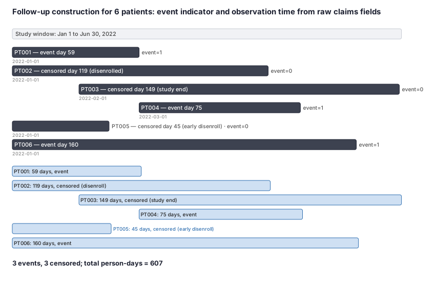
Six new users of a diabetes drug are followed from their first prescription (the index date) until a hospitalization for hypoglycemia (the event) or until they leave observation — either by disenrolling from their insurance plan or when the study data are collected on June 30, 2022. The analyst must build the (follow_up_days, event) pair for each patient from the raw date fields before fitting a Kaplan-Meier curve. Three patients have the event; three are censored for different reasons, illustrating administrative censoring, informative early disenrollment, and end-of-study administrative censoring in a single cohort.

Dataset

Raw date fields as they appear in a claims extract. A tilde (~) means no date recorded for that field. The study_end is June 30, 2022 for all patients. The analyst must compute follow_up_days and event from these five columns.

person_id	index_date	event_date	disenroll_date	study_end
PT001	2022-01-01	2022-03-01		2022-06-30
PT002	2022-01-01		2022-04-30	2022-06-30
PT003	2022-02-01			2022-06-30
PT004	2022-03-01	2022-05-15		2022-06-30
PT005	2022-01-01		2022-02-15	2022-06-30
PT006	2022-01-01	2022-06-10		2022-06-30

Steps

Result

Follow-up construction complete. PT001: 31+28 = 59 days, event = 1. PT002: 31+28+31+29 = 119 days, event = 0 (plan disenrollment). PT003: 28+31+30+31+29 = 149 days, event = 0 (study end). PT004: 31+30+14 = 75 days, event = 1. PT005: 31+14 = 45 days, event = 0 (early disenrollment). PT006: 31+28+31+30+31+9 = 160 days, event = 1. Total person-days: 59+119+149+75+45+160 = 607. Event fraction: 3/6 = 0.50. These six rows are the direct input to KaplanMeierFitter (Python), survfit() (R), or PROC LIFETEST (SAS).

Timeline Spec

Title

Follow-up construction for 6 patients: event indicator and observation time from raw claims fields

Window

Start: 2022-01-01
End: 2022-06-30
Label: Study window: Jan 1 to Jun 30, 2022

Events

Label
PT001 — event day 59
Start
2022-01-01
Length Days
59
Quantity
event=1
Label
PT002 — censored day 119 (disenrolled)
Start
2022-01-01
Length Days
119
Quantity
event=0
Label
PT003 — censored day 149 (study end)
Start
2022-02-01
Length Days
149
Quantity
event=0
Label
PT004 — event day 75
Start
2022-03-01
Length Days
75
Quantity
event=1
Label
PT005 — censored day 45 (early disenroll)
Start
2022-01-01
Length Days
45
Quantity
event=0
Label
PT006 — event day 160
Start
2022-01-01
Length Days
160
Quantity
event=1

Spans

Kind
followup
Start
2022-01-01
End
2022-03-01
Label
PT001: 59 days, event
Kind
followup
Start
2022-01-01
End
2022-04-30
Label
PT002: 119 days, censored (disenroll)
Kind
followup
Start
2022-02-01
End
2022-06-30
Label
PT003: 149 days, censored (study end)
Kind
followup
Start
2022-03-01
End
2022-05-15
Label
PT004: 75 days, event
Kind
followup
Start
2022-01-01
End
2022-02-15
Label
PT005: 45 days, censored (early disenroll)
Kind
followup
Start
2022-01-01
End
2022-06-10
Label
PT006: 160 days, event

Result

Label: 3 events, 3 censored; total person-days = 607
Value: 607

Runnable example

python implementation

Demonstrates the primitive (follow_up_days, event) construction from raw claims-like date fields using pandas, then fits a Kaplan-Meier curve with lifelines. The key operation is computing censor_date = min(disenroll_date, study_end) and resolving whether...

import pandas as pd
from lifelines import KaplanMeierFitter

# ── Raw claims-like fields: as they appear in a cohort extract ──
data = pd.DataFrame({
    "person_id":      ["PT001","PT002","PT003","PT004","PT005","PT006"],
    "index_date":     pd.to_datetime(["2022-01-01","2022-01-01","2022-02-01",
                                      "2022-03-01","2022-01-01","2022-01-01"]),
    "event_date":     pd.to_datetime(["2022-03-01", None, None,
                                      "2022-05-15", None, "2022-06-10"]),
    "disenroll_date": pd.to_datetime([None, "2022-04-30", None,
                                      None, "2022-02-15", None]),
    "study_end":      pd.to_datetime(["2022-06-30"] * 6),
})

# ── PRIMITIVE CONSTRUCTION: (follow_up_days, event) from raw date fields ──

# Step 1: censoring date = earliest of disenrollment or study end (ignore NaT)
data["censor_date"] = data[["disenroll_date", "study_end"]].min(axis=1)

# Step 2: event occurred if event_date exists AND is on or before censor_date
data["had_event"] = (
    data["event_date"].notna() &
    (data["event_date"] <= data["censor_date"])
)

# Step 3: end_date = event_date if event, else censor_date
data["end_date"] = data["event_date"].where(data["had_event"], data["censor_date"])

# Step 4: follow-up time in days from index to end
data["follow_up_days"] = (data["end_date"] - data["index_date"]).dt.days

# Step 5: binary event indicator (1 = event observed, 0 = censored)
data["event"] = data["had_event"].astype(int)

print("Follow-up table:")
print(data[["person_id", "follow_up_days", "event"]].to_string(index=False))
# Expected output:
#  person_id  follow_up_days  event
#      PT001              59      1
#      PT002             119      0
#      PT003             149      0
#      PT004              75      1
#      PT005              45      0
#      PT006             160      1

# ── Kaplan-Meier estimate ──
kmf = KaplanMeierFitter()
kmf.fit(
    durations=data["follow_up_days"],
    event_observed=data["event"],
    label="New-user cohort"
)
print(f"\nMedian survival time: {kmf.median_survival_time_} days")
print(f"95% CI: {kmf.confidence_interval_median_.values}")
# Note: with only 6 patients the CI will be wide; this illustrates the construction,
# not a powered survival estimate. In production, verify event_date <= censor_date
# strictly (not <=) if same-day events and censorings need disambiguation.

r implementation

Demonstrates the primitive Surv(time, event) construction from raw claims-like date fields in base R, then fits a Kaplan-Meier curve with survfit(). The pmin() call implements censor_date = min(disenroll_date, study_end), and the event indicator is built...

library(survival)

# ── Raw claims-like fields ──
df <- data.frame(
  person_id      = c("PT001","PT002","PT003","PT004","PT005","PT006"),
  index_date     = as.Date(c("2022-01-01","2022-01-01","2022-02-01",
                             "2022-03-01","2022-01-01","2022-01-01")),
  event_date     = as.Date(c("2022-03-01", NA, NA,
                             "2022-05-15", NA, "2022-06-10")),
  disenroll_date = as.Date(c(NA, "2022-04-30", NA, NA, "2022-02-15", NA)),
  study_end      = as.Date(rep("2022-06-30", 6)),
  stringsAsFactors = FALSE
)

# ── PRIMITIVE CONSTRUCTION: Surv(time, event) from raw date fields ──

# Step 1: censoring date = earliest of disenrollment or study end (na.rm ignores NA)
df$censor_date <- pmin(df$disenroll_date, df$study_end, na.rm = TRUE)

# Step 2: event occurred if event_date exists AND is on or before censor_date
df$event <- as.integer(!is.na(df$event_date) & df$event_date <= df$censor_date)

# Step 3: end_date = event_date if event, else censor_date
df$end_date <- as.Date(
  ifelse(df$event == 1L, as.character(df$event_date), as.character(df$censor_date))
)

# Step 4: follow-up time in days
df$follow_up_days <- as.numeric(df$end_date - df$index_date)

cat("Follow-up table:\n")
print(df[, c("person_id", "follow_up_days", "event")])
# Expected output:
#   person_id follow_up_days event
# 1     PT001             59     1
# 2     PT002            119     0
# 3     PT003            149     0
# 4     PT004             75     1
# 5     PT005             45     0
# 6     PT006            160     1

# ── Surv() object and Kaplan-Meier ──
# Surv(time, event): event = 1 means observed; event = 0 means censored (the default coding)
surv_obj <- Surv(time = df$follow_up_days, event = df$event)
km_fit   <- survfit(surv_obj ~ 1, data = df)

print(summary(km_fit))
# The summary shows survival probability at each event time.
# With n=6 and 3 events, CIs are wide but the construction is identical to large cohorts.

# Median survival time with 95% CI (Hall-Wellner or log-log bands)
cat(sprintf("\nMedian: %g days  95%% CI: %g-%g\n",
            quantile(km_fit, 0.5)$quantile,
            quantile(km_fit, 0.5)$lower,
            quantile(km_fit, 0.5)$upper))