Study Time Windows: Baseline, Observation, and Outcome Windows

In plain language

Every RWE study is built around a patient's personal "day zero" — the date they first filled a new prescription or received a new diagnosis — and a set of named time windows that surround that date. Before day zero, there is a lookback window where you confirm the patient had no prior use of the drug and measure their background health. After day zero there is sometimes a short excluded zone (an induction window) where events don't yet count because the drug hasn't had time to act, and then the main outcome window where you watch for the event you care about. Getting these windows right — and making sure they only cover time when the patient was actually enrolled in their health plan — is the foundational step that every valid RWE study depends on.

Study time windows are the full temporal skeleton of an RWE study

Every claim, diagnosis, fill, lab, or utilization record is only analytically meaningful once it is assigned to a named window: is it evidence of a past condition (baseline), evidence the patient is being captured at all (observation), an event that should not yet be attributed to exposure (induction), or an event that counts as an outcome (risk window)? Newcomers often skip this architecture and write eligibility and outcome queries without fully specifying the temporal logic, producing cohorts whose time-zero is misaligned, whose covariates bleed past index, or whose outcome windows extend beyond real observability. This entry is the map: it names every window in a typical RWE timeline, shows how they assemble around the index date, and routes the reader to the deep concepts that govern each one.

The index date (time zero): the anchor

Every other window is defined relative to the index date, so getting this right is the first obligation of any cohort definition. The index date is the study's time-zero — the moment the patient "enters" the study's at-risk clock. In a new-user drug cohort it is the date of the first qualifying prescription fill after all eligibility conditions are met. In an incident-disease cohort it is the date of the first qualifying diagnosis. In a target-trial emulation it is the date of the first "protocol-eligible" assignment.

Three properties of a valid index date deserve explicit statement in every protocol. First, it must be the first qualifying event — which is only meaningful after a washout has confirmed the patient was not already using the drug/had the diagnosis before entering the study. Second, it must fall inside an observable window: the patient must be enrolled in a health plan (or actively under data capture in an EHR/registry) at the index date itself. Third, it must be assigned before the analysis sees outcomes — any rule that requires a patient to survive long enough to receive a confirming event after what is called "time zero" creates immortal time bias (`immortal-time-bias-handling`).

The index date is the single most consequential specification in an RWE study. Every window below is described as an offset from it.

Baseline / lookback / covariate assessment window

The baseline window is the pre-index span — ending either the day before the index date (the standard convention, noted "index_date − 1") or on the index date itself — during which covariates are measured, eligibility conditions are evaluated, and (as a special case) the washout is executed. Typical lengths are 180 days and 365 days for claims, though longer windows (730 days) appear for conditions with long coding lags (chronic kidney disease, depression). The canonical formulation: a patient contributes to the 365-day baseline window if they are continuously enrolled from `index_date − 365` through `index_date − 1`.

Three distinct purposes are bundled in the same pre-index span, and conflating them is a common protocol error (see `washout-clean-lookback-period-rwe`). The washout use is exclusionary: require absence of the study drug (and comparator, in an active-comparator design) during the window, so that only new (incident) users enter the cohort. The covariate measurement use is additive: count the presence of diagnoses, fills, procedures, and labs during the window to build the baseline covariate vector. The eligibility use is confirmatory: verify the required diagnosis was or was not present, verify the required enrollment span was covered, verify that competing treatments were absent.

Two design choices dominate the baseline window's bias profile. The first is fixed-length vs all-available history. A fixed-length baseline (e.g., exactly 365 days) gives comparable covariate ascertainment across every patient regardless of how long they have been enrolled — a key advantage for propensity-score and outcome-model balance. An all-available baseline captures more true chronic conditions (a hypertension diagnosis coded once five years ago would be missed by a 365-day window) but inflates covariate counts for long-enrollees, inducing differential measurement by arm if one arm skews toward longer enrollment history. The second is endpoint: does the baseline window end `index_date − 1` (the day before the index date) or does it include the index date itself? Including same-day events in the baseline is the source of the classic off-by-one error: a patient can appear to have both a baseline comorbidity recorded on the index date and an outcome recorded on the index date, even though they entered and had a simultaneous event — whether that counts as a baseline condition, a mediator, or an event depends on the exact time-of-day of each record, which claims do not carry. Standard practice ends the baseline at `index_date − 1`.

The baseline window is only valid if the patient is enrolled and observable across its full span. "No prior fill in 365 days" is a confident new-user designation only if the data actually observed the patient for all 365 days. Enrollment must cover the baseline window completely (`continuous-enrollment-observable-time-rwe`).

Observation window / observable time

The observation window is the span during which the data source is actually capturing the patient's healthcare encounters. It is not a study-analytic window but a data-availability constraint: the fundamental precondition that makes any other window meaningful. In claims, it is operationalized as the patient's continuous enrollment span(s) with the relevant benefits (medical + pharmacy for drug studies, at minimum). In OMOP CDM studies, it is the `observation_period` table (`omop-observation-period-rwe`). In EHR, it is inferred from encounter density.

The critical inferential principle: absence of a code within the observation window can be interpreted as absence of the event. Outside the observation window, silence is missingness — it cannot be read as a clean record. This asymmetry governs every window that follows. If a patient's enrollment ends on 2022-06-15, an outcome that occurs on 2022-06-20 does not appear in the data — it is not a non-event, it is a censoring event. The analysis must treat the patient as censored at disenrollment, not followed through the outcome.

Gaps in enrollment break the observation window. Most protocols allow a small gap tolerance — commonly 30 or 45 days — across which enrollment is assumed continuous (the gap might represent a brief plan switch, an administrative lag, or a formulary change). Gaps wider than the tolerance split the observation window into separate observable spans. A patient's time-at-risk and baseline lookback must both be restricted to the observable spans.

Induction / lag / blackout window

Immediately after the index date there is often a span of days during which outcomes are excluded from the primary analysis. This post-index exclusion zone goes by several names in the literature: induction window, lag period, blanking period, blackout window. Its purpose is biologically and analytically distinct from the baseline: rather than cleaning the pre-index history, it cleans the post-index outcome window of events that could not plausibly have been caused by the exposure because not enough time has elapsed (see `exposure-lag-induction-latency-window-rwe`).

Two distinct rationales drive the induction window. The first is protopathic bias / reverse causation: if a patient was already developing the outcome condition when they received the first prescription, the early post-index outcomes reflect pre-existing disease, not drug effect. A 30-day or 90-day induction window excludes these events. The second is biological latency: some outcomes require a minimum biological delay before they can manifest (e.g., drug-induced liver injury typically requires weeks of exposure; cancer chemoprevention requires months or years). An induction window shorter than the true minimum latency will bias toward the null, so the length must be justified by the pharmacological or disease mechanism.

In a new-user cohort, the induction window runs from the index date through `index_date + induction_days − 1` (e.g., days 0–29 for a 30-day induction). Events within this window are excluded from the outcome count but the patient is not censored — they continue contributing to person-time for the outcome window that follows. (Contrast: if a patient dies during the induction window, their follow-up truly ends; the induction window excludes only the non-fatal outcome count, not follow-up itself.)

Outcome / risk / assessment window

The outcome window is the post-index span during which events are attributed to exposure. In a time-to-event (survival) analysis it starts immediately after the induction window ends (or at the index date, if no induction is applied) and continues until the first of: (a) the outcome event, (b) disenrollment/end of observation, (c) death (a competing event or a censoring event depending on the outcome), or (d) an administrative end-of-data date. In a fixed-window utilization or cost study (e.g., per-patient-per-month costs over a 12-month window post-index), the outcome window has a hard calendar stop at `index_date + 365`.

The outcome window's start and end determine the estimand. An intention-to-treat (ITT) outcome window starts at time zero and runs regardless of whether the patient continued on the original drug — it measures the effect of initiating a treatment strategy. An as-treated outcome window builds on- treatment time by stitching supply intervals, applying a grace period, and censoring when the patient discontinues or switches — it measures the effect of remaining on the drug (`as-treated-risk-window-construction-rwe`). The two are not interchangeable and should rarely be mixed in the same analysis without explicit justification.

Death as a censoring event vs a competing event is a critical distinction in the outcome window (`mortality-source-hierarchy-rwe`). For an all-cause mortality endpoint, death is the outcome and the outcome window ends at death. For any other endpoint (hospitalization, fracture, stroke), death is a competing event — a patient who dies can no longer experience the outcome, so simple censoring at death biases the cumulative-incidence estimate (Fine-Gray or cause-specific hazard analysis is required). Additionally, the granularity of the death date matters: if the mortality source (National Death Index, Social Security Death Master File) provides only month-and-year of death, not day, the death date is often coded as the last day of the month. This day-level error shifts the censoring date by up to 30 days and can meaningfully bias short-window estimands (e.g., 30-day mortality). Protocols must specify which mortality source is used and how day-level imprecision is handled.

Follow-up period: the umbrella

"Follow-up period" is the colloquial umbrella for everything after the index date: induction + outcome window combined. A given calendar date can fall in a different window for different patients because follow-up is patient-anchored to each patient's index date, not to the calendar. Patient A, whose index date is 2020-01-15, and Patient B, whose index date is 2021-07-03, may both appear in the 2021 claims data in their outcome windows, but they entered the cohort at different times — the calendar alignment is irrelevant; what matters is person-time-since-index. This is why incidence rates are always expressed in units of person-time (events per 100 person-years), not per calendar year.

The assembled picture: the design-diagram convention

The most effective protocol artifact for communicating all windows at once is the graphical design diagram standardized by Schneeweiss et al. (2019). The diagram draws each named window as a labeled horizontal bar on a single timeline anchored at the index date, with the direction of time left-to-right and the index date marked with a vertical line. A complete design diagram carries: (1) the continuous- enrollment span (the envelope), (2) the washout/baseline window (pre-index, shaded gray), (3) the index date (vertical milestone), (4) the induction/lag window (post-index, cross-hatched), and (5) the outcome/follow-up window (post-induction, clear or colored by arm). Every protocol and SAP should carry one. A protocol that can describe its time windows verbally but cannot draw them is a protocol that has not fully specified them.

Pros, cons, and trade-offs — specific and comparative

• Fixed-length baseline vs all-available lookback: A fixed-length baseline (365 days) standardizes

• ITT outcome window vs as-treated risk window: ITT is cleaner, avoids informative-censoring bias,

• Induction window present vs absent: Induction windows remove protopathic bias and biologically

• Hard administrative cap on follow-up vs open-ended follow-up: A hard 12-month outcome window

When to use

This architecture applies to every longitudinal database study without exception. Any time a cohort is built from claims, EHR records, registry data, or linked sources, the analyst must specify an index date rule, a baseline window, an observation window, and an outcome window — whether or not those names are used. Failure to specify any one of them does not mean it is absent; it means it has been implicitly chosen (often badly) by whatever default behavior the extraction code happens to produce. Use this framework explicitly as the first design artifact, before any eligibility SQL or analysis code is written.

When NOT to use — and when it is actively misleading or dangerous

• Do not apply a baseline covariate window that extends past the index date. Any diagnosis,

• Do not define the outcome window so it extends past the enrollment-verified span. An outcome

• Do not treat the induction window as an eligibility filter. Requiring that a patient survive

• Do not use month-year death dates as day-precise censoring without acknowledging the error.

• Do not use a single enrollment span when the patient has multiple non-contiguous spans.

Pitfalls at the window boundaries

Immortal time from misaligned windows. The most dangerous version: the index date is set at a diagnosis date, but eligibility also requires a subsequent prescription fill. Every patient who qualified was event-free from their diagnosis to their fill — that interval, attributed to the "treated" group as at-risk follow-up, is immortal. Fix: set the index date at the first fill, not the diagnosis (`immortal-time-bias-handling`).

Baseline covariates measured after index. A propensity score that includes any diagnosis, procedure, or lab recorded on or after the index date adjusts for a mediator or post-treatment confounder and introduces selection bias. Run a simple check: every covariate look-up date must satisfy `event_date < index_date`.

Outcome window extending past disenrollment. Events that occur after enrollment ends are invisible in claims but are not non-events. If the outcome window is not capped at the enrollment end date, disenrolled follow-up days inflate the person-time denominator without contributing events — rates are biased downward, and differential rates of disenrollment across arms become differential censoring.

Month-granularity death dates truncating follow-up. For analyses near the date of death — hospice cost, end-of-life utilization, 30-day readmission — a month-only death date from the SSDI or NDI can place the death on the wrong calendar day, altering the length of every follow-up window that terminates at death. See `mortality-source-hierarchy-rwe` for how to build and validate the composite death date.

Differential enrollment duration by arm creating asymmetric windows. If one drug arm skews toward older Medicare patients with longer enrollment histories and the other arm skews toward younger commercial enrollees who churn more, the two arms will have different baseline window lengths if all-available lookback is used, different rates of induction-window events lost (because survival differs), and different follow-up censoring patterns. Fix: use a fixed-length baseline and report enrollment-duration diagnostics stratified by arm.

Worked example

Scenario

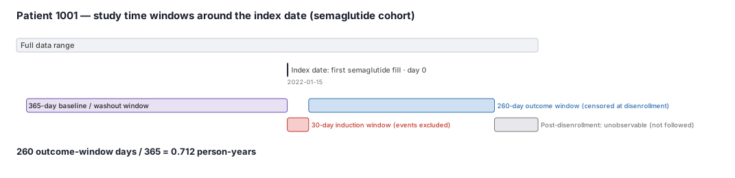
A researcher is building a new-user cohort of adults with type 2 diabetes who start a GLP-1 receptor agonist. One patient — call her Patient 1001 — first fills semaglutide on 2022-01-15. The protocol specifies a 365-day baseline window ending the day before index, a 30-day induction window, and an outcome window that runs from day 31 through disenrollment or end of data (2022-12-31). The enrollment record shows the patient was continuously enrolled from 2021-01-01 through 2022-10-31, then disenrolled. We want to (a) confirm the patient passes the baseline enrollment requirement, (b) identify the exact calendar dates of each window, and (c) compute the length of the outcome window she actually contributes.

Dataset

Patient 1001's enrollment span and index date — the raw inputs an analyst would use.

Steps

• Baseline window: index_date - 365 days through index_date - 1 day = 2021-01-15 through 2022-01-14. Length = 365 days.

• Enrollment check: enrollment_start (2021-01-01) <= baseline_start (2021-01-15) and enrollment_end (2022-10-31) >= index_date (2022-01-15). Both conditions are met, so the patient has fully observable pre-index history. The washout and covariate windows are valid.

• Induction window: index_date through index_date + 29 days = 2022-01-15 through 2022-02-13. Length = 30 days. Events in this window are excluded from the outcome count.

• Outcome window start: induction_end + 1 day = 2022-02-14.

• Outcome window end: the earlier of enrollment_end (2022-10-31) and end_of_data (2022-12-31) is 2022-10-31. The patient was censored at disenrollment, not at the data cutoff.

• Outcome window length: 2022-02-14 through 2022-10-31. Days = (2022-10-31) - (2022-02-14) + 1 = 260 days.

Result

Patient 1001 contributes a 365-day baseline window (2021-01-15 through 2022-01-14), passes the enrollment check, has a 30-day induction window (2022-01-15 through 2022-02-13), and contributes 260 days of outcome-window follow-up (2022-02-14 through 2022-10-31) before being censored at disenrollment. She is NOT followed through end of data because her enrollment ended before 2022-12-31. Total person-time in the outcome window = 260 / 365 = 0.712 person-years.

Timeline Spec

Title

Patient 1001 — study time windows around the index date (semaglutide cohort)

Window

Start

2021-01-01

End

2022-12-31

Label

Full data range

Events

• Label

  Index date: first semaglutide fill

  Start

  2022-01-15

  Length Days

  1

  Quantity

  day 0

Spans

• Kind

  washout

  Start

  2021-01-15

  End

  2022-01-14

  Label

  365-day baseline / washout window

• Kind

  gap

  Start

  2022-01-15

  End

  2022-02-13

  Label

  30-day induction window (events excluded)

• Kind

  followup

  Start

  2022-02-14

  End

  2022-10-31

  Label

  260-day outcome window (censored at disenrollment)

• Kind

  unexposed

  Start

  2022-11-01

  End

  2022-12-31

  Label

  Post-disenrollment: unobservable (not followed)

Result

Label

260 outcome-window days / 365 = 0.712 person-years

Value

0.712

Runnable example

from datetime import date, timedelta
from dataclasses import dataclass

@dataclass
class StudyWindows:
    """All time-window boundaries for one patient in a new-user RWE cohort."""
    person_id: int
    index_date: date          # day 0 (first qualifying fill/diagnosis)
    enrollment_start: date    # first day of observable coverage
    enrollment_end: date      # last day of observable coverage (inclusive)
    end_of_data: date         # hard data cutoff (inclusive)
    lookback_days: int = 365  # length of baseline/washout window
    induction_days: int = 30  # days post-index excluded from outcome count

def compute_windows(p: StudyWindows) -> dict:
    """
    Derive every named window for one patient.

    Baseline convention: ends index_date - 1 (not index_date), avoiding
    the same-day off-by-one where a condition coded on index day would
    appear in both baseline and potential-outcome.

    Outcome window: runs induction_end + 1 through min(enrollment_end, end_of_data).
    Day count uses inclusive endpoints: length = (end - start).days + 1.
    """
    # --- Baseline window (pre-index, inclusive on both ends) ---
    baseline_start = p.index_date - timedelta(days=p.lookback_days)
    baseline_end   = p.index_date - timedelta(days=1)   # day BEFORE index
    baseline_days  = (baseline_end - baseline_start).days + 1  # = lookback_days

    # --- Enrollment coverage check for baseline ---
    # The patient must have been continuously enrolled across the ENTIRE baseline window.
    # If enrollment_start > baseline_start the washout window is not fully observable.
    baseline_covered = (
        p.enrollment_start <= baseline_start and
        p.enrollment_end   >= p.index_date
    )

    # --- Induction window (post-index, events excluded from outcome count) ---
    # Runs from index_date (inclusive) through index_date + induction_days - 1.
    induction_start = p.index_date
    induction_end   = p.index_date + timedelta(days=p.induction_days - 1)
    induction_days_actual = (induction_end - induction_start).days + 1

    # --- Outcome / follow-up window ---
    # Starts the day after the induction window ends; capped at the earlier of
    # enrollment_end and end_of_data. If the cap falls before the start, the
    # patient contributes no observable outcome-window time (censored during induction).
    outcome_start = induction_end + timedelta(days=1)
    outcome_end   = min(p.enrollment_end, p.end_of_data)
    if outcome_end < outcome_start:
        outcome_days = 0
        outcome_person_years = 0.0
    else:
        outcome_days = (outcome_end - outcome_start).days + 1
        outcome_person_years = outcome_days / 365.25

    return {
        "person_id":              p.person_id,
        "baseline_start":         baseline_start,
        "baseline_end":           baseline_end,
        "baseline_days":          baseline_days,
        "baseline_covered":       baseline_covered,
        "index_date":             p.index_date,
        "induction_start":        induction_start,
        "induction_end":          induction_end,
        "induction_days":         induction_days_actual,
        "outcome_start":          outcome_start,
        "outcome_end":            outcome_end,
        "outcome_days":           outcome_days,
        "outcome_person_years":   round(outcome_person_years, 4),
        "censored_at_disenroll":  p.enrollment_end < p.end_of_data,
    }

# ── Demonstration with Patient 1001 from the worked example ──
p1001 = StudyWindows(
    person_id       = 1001,
    index_date      = date(2022, 1, 15),
    enrollment_start= date(2021, 1,  1),
    enrollment_end  = date(2022, 10, 31),
    end_of_data     = date(2022, 12, 31),
    lookback_days   = 365,
    induction_days  = 30,
)
w = compute_windows(p1001)
print("Baseline window: ", w["baseline_start"], "to", w["baseline_end"],
      f"({w['baseline_days']} days)")
print("Baseline covered:", w["baseline_covered"])
print("Induction window:", w["induction_start"], "to", w["induction_end"],
      f"({w['induction_days']} days)")
print("Outcome window:  ", w["outcome_start"], "to", w["outcome_end"],
      f"({w['outcome_days']} days = {w['outcome_person_years']} person-years)")
print("Censored at disenroll:", w["censored_at_disenroll"])
# Expected output:
# Baseline window:  2021-01-15 to 2022-01-14 (365 days)
# Baseline covered: True
# Induction window: 2022-01-15 to 2022-02-13 (30 days)
# Outcome window:   2022-02-14 to 2022-10-31 (260 days = 0.7119 person-years)
# Censored at disenroll: True

# Study time window computation for a new-user RWE cohort
# Base-R Date arithmetic: dates are numeric days since 1970-01-01;
# subtraction gives the number of days between two dates (exclusive end).
# Inclusive length: (end - start) + 1L.

compute_windows_r <- function(
    person_id,
    index_date,        # as.Date("YYYY-MM-DD")
    enrollment_start,
    enrollment_end,
    end_of_data,
    lookback_days = 365L,
    induction_days = 30L
) {
  # --- Baseline window ---
  baseline_start <- index_date - lookback_days
  baseline_end   <- index_date - 1L           # day BEFORE index (off-by-one convention)
  baseline_length <- as.integer(baseline_end - baseline_start) + 1L  # == lookback_days

  # --- Enrollment coverage check ---
  # Patient must be enrolled across the ENTIRE baseline window.
  baseline_covered <- (enrollment_start <= baseline_start) &
                      (enrollment_end   >= index_date)

  # --- Induction window ---
  induction_start <- index_date
  induction_end   <- index_date + induction_days - 1L
  induction_length <- as.integer(induction_end - induction_start) + 1L

  # --- Outcome window ---
  outcome_start <- induction_end + 1L
  outcome_end   <- min(enrollment_end, end_of_data)  # cap at earlier of disenroll / data end
  outcome_length <- if (outcome_end >= outcome_start) {
    as.integer(outcome_end - outcome_start) + 1L
  } else {
    0L  # patient disenrolled during or before the induction window
  }
  outcome_person_years <- round(outcome_length / 365.25, 4)

  data.frame(
    person_id             = person_id,
    baseline_start        = baseline_start,
    baseline_end          = baseline_end,
    baseline_days         = baseline_length,
    baseline_covered      = baseline_covered,
    index_date            = index_date,
    induction_start       = induction_start,
    induction_end         = induction_end,
    induction_days        = induction_length,
    outcome_start         = outcome_start,
    outcome_end           = outcome_end,
    outcome_days          = outcome_length,
    outcome_person_years  = outcome_person_years,
    censored_at_disenroll = enrollment_end < end_of_data,
    stringsAsFactors      = FALSE
  )
}

# -- Patient 1001 from the worked example --
w <- compute_windows_r(
  person_id        = 1001L,
  index_date       = as.Date("2022-01-15"),
  enrollment_start = as.Date("2021-01-01"),
  enrollment_end   = as.Date("2022-10-31"),
  end_of_data      = as.Date("2022-12-31"),
  lookback_days    = 365L,
  induction_days   = 30L
)
print(w[, c("baseline_start", "baseline_end", "baseline_days",
            "baseline_covered", "induction_end", "outcome_start",
            "outcome_end", "outcome_days", "outcome_person_years")])
# Expected:
# baseline_start: 2021-01-15
# baseline_end:   2022-01-14   baseline_days: 365  baseline_covered: TRUE
# induction_end:  2022-02-13
# outcome_start:  2022-02-14   outcome_end: 2022-10-31
# outcome_days:   260          outcome_person_years: 0.7119