Multi-State Models
A framework that represents a patient's disease history as movement between a finite set of states (e.g., Stable, Progressed, Dead) connected by allowed transitions, estimates the transition intensities (cause-specific hazards) that govern each move, and assembles them with the Aalen-Johansen estimator into transition probabilities - the chance of occupying each state at a future time given the state occupied now - thereby generalizing standard survival analysis and competing risks to repeated, intermediate, and possibly reversible events.
On this page
A multi-state model tracks patients as they move between a small set of health states over time - for example Stable, Progressed, and Dead - and estimates the chance of being in each state at any future time. Instead of studying a single yes/no outcome, you study every allowed move (a transition) and the rate at which each move happens. From those rates, the Aalen-Johansen estimator builds the probability that a patient who starts Stable is Stable, Progressed, or Dead one or two years later. Competing risks is just the special case where the only moves are out of the starting state into a few final (absorbing) states.
Standard survival analysis asks one question - time to a single event - and competing risks extends it to "time to the first of several mutually exclusive events." A multi-state model is the natural generalization of both: it represents a patient's history as a token sitting in one of a finite set of states and moving along allowed transitions between them over time. Cancer patients move Stable -> Progressed -> Dead; transplant patients move Transplanted -> Graft-failure -> Dead, or back to Re-transplant; HIV patients move across CD4 strata.
Each arrow in the state diagram is governed by a transition intensity (a hazard for that specific move, possibly depending on time and covariates), and the whole object answers questions that a single Cox model cannot: what is the probability a patient who is progression-free today will be alive-with-progression in two years? That quantity - state occupancy / transition probability - is the deliverable, and it is exactly what health-technology-assessment cost-effectiveness models consume.
The machinery, in order
(1) States and transitions. Declare the states and the transition matrix (which moves are allowed). States are transient (you can leave) or absorbing (death - you cannot leave). (2) Transition intensities. For each allowed transition s -> s', the instantaneous rate of that move among those currently in state s. These are estimated transition-by-transition: nonparametrically (Nelson-Aalen cumulative hazards per transition) or with a transition-specific Cox model (stratify the baseline hazard by transition; let covariate effects differ by transition).
(3) Transition probabilities via Aalen-Johansen. The intensities are assembled into the K x K matrix P(s, t) of probabilities of moving from each state at time s to each state at time t. Aalen-Johansen is the estimator: it is a product-integral - a matrix product, over all event times u in (s, t], of (I + dA(u)) where dA(u) holds the estimated transition increments at u.
With no censoring it reduces to the empirical fraction of the cohort occupying each state; its real value is that it correctly reweights the at-risk sets under right-censoring, which a naive state-occupancy tally does not. Competing risks (cumulative incidence functions) is the special case with one transient starting state and several absorbing states and no onward moves - Aalen-Johansen there is exactly the cumulative-incidence estimator.
The two assumptions that define your model
Markov vs semi-Markov. In a Markov model the transition intensity out of a state depends only on the current state and the time since study origin (clock-forward) - not on how long the patient has been in the current state, nor how they got there. In a semi-Markov (clock-reset) model the intensity depends on the time since entering the current state (the clock resets to zero at each transition).
For a Progressed -> Dead transition this is the crux: clock-forward says mortality risk tracks calendar time from diagnosis; clock-reset says it tracks duration of progressed disease (usually the more clinically honest choice). A homogeneous Markov model further assumes constant intensities (the engine of classic HTA Markov cohort models with fixed cycle transition probabilities); the nonparametric multi-state model here makes no such constancy assumption.
Pros, cons, and trade-offs
(specific and comparative).
- vs competing-risks-cause-specific-fine-gray-rwe (the special case): Multi-state strictly contains competing risks - add intermediate states and onward transitions and you have it. Prefer the competing-risks framing when every event is terminal and you only need cumulative incidence of first events; prefer the full multi-state model the moment an intermediate, non-absorbing event (progression, relapse, hospitalization, graft failure) matters and you want the probability of currently being in that intermediate state, or the effect of passing through it on downstream risk. A Fine-Gray subdistribution model gives you one cumulative incidence curve; it cannot tell you how many patients are alive with progression right now.
- vs partitioned-survival-models-rwe (the HTA debate): Partitioned survival (PartSA) reconstructs state occupancy by subtracting independently fitted overall-survival and progression-free-survival curves - "alive-and-progressed" = OS minus PFS. It is simple and standard in oncology dossiers but structurally incoherent: the three state-membership curves are not constrained to come from a consistent transition process, so the implied post-progression survival is an output, not a modeled quantity, and can behave implausibly in extrapolation. A multi-state (state-transition) model fits the Progressed -> Dead transition directly, so post-progression survival is governed by an estimated hazard and the curves are internally consistent by construction. Prefer PartSA only when data are too thin to estimate the intermediate transition or when a regulator/HTA precedent demands it; prefer the multi-state model whenever post-progression survival, treatment switching at progression, or coherent long-term extrapolation drives the cost-effectiveness result (NICE TSD 19 makes exactly this recommendation).
- vs a single Cox model on a composite or first event (cox-ph-regression): One Cox model collapses a rich history into a single time-to-event and throws away the intermediate structure. The multi-state model keeps it, at the cost of estimating several transition-specific hazards (more parameters, sparser at-risk sets on the later transitions) and of having to choose and defend the Markov/semi-Markov and clock assumptions.
When NOT to use - and when it is actively misleading
- The illness-death model with an unverified Markov assumption. The canonical three-state structure (Healthy -> Ill -> Dead, with a direct Healthy -> Dead arrow) is the workhorse, but the Ill -> Dead intensity is almost never truly clock-forward Markov - mortality after progression depends on duration of progressed disease, not calendar time from origin. Fitting a Markov Ill -> Dead transition when the process is semi-Markov biases the transition probabilities and the extrapolated post-progression survival. Test it (e.g., add time-in-state as a covariate) or fit clock-reset.
- Sparse late transitions. The onward transitions (Progressed -> Dead) are estimated only among the subset who reached the intermediate state, so the at-risk set is small and the hazard is noisy. Over-parameterizing transition-specific covariate effects on a thin transition produces unstable estimates; consider sharing baseline hazards or covariate effects across transitions when justified.
- Treating Aalen-Johansen state occupancy as if it adjusted for confounding. Aalen-Johansen is a descriptive / prognostic estimator of transition probabilities in the observed cohort. Comparing arms by their multi-state curves is not a causal contrast unless you have handled confounding (e.g., weight the transitions, or embed the multi-state model in a target-trial emulation). A naive arm comparison of state occupancy inherits all the usual confounding-by-indication of observational data.
- Interval-censored state transitions. When the intermediate state is only observed at scheduled visits (you see that progression happened between two visits, not when), the exact-transition-time machinery of Aalen-Johansen does not apply; a panel/Markov interval-censored model (e.g., a continuous-time Markov chain fit to panel data) is required instead.
Data-source operational depth
- Claims: States must be constructed from codes - "Progressed" has no field; it is proxied by a regimen switch, a new line of therapy, a radiotherapy/secondary-malignancy code, or hospice enrollment, and "Dead" needs a death source (inpatient discharge disposition, linked death index) because pharmacy/medical claims do not record outpatient death. Transition times are interval-flavored (you see the claim, not the clinical event), so the apparent transition date is a coding date, not the biological one.
- EHR: Richer state definition (labs, vitals, problem list, oncology flowsheets, RECIST in structured or note-derived fields) and finer transition timing, but death and out-of-system transitions are missed when the patient leaves the network - that informative loss-to-follow-up censors the later transitions non-randomly.
- Registry: Disease registries (cancer, transplant) are the cleanest substrate - states and transition dates are adjudicated prospectively, which is why the illness-death and competing-risks literature grew up on them - but cause-of-death and post-exit transitions may still need linkage.
- Linked claims-EHR-registry: The ideal: registry/EHR for adjudicated state definitions and transition timing, claims for treatment-switch proxies and continuity, a death index for the absorbing state. Reconcile the differing transition dates across sources before building the long-format risk sets.
Interpreting the output
An Aalen-Johansen multi-state model (stable → progressed → dead) returns at year 2: P(Stable) = 0.73, P(Progressed) = 0.15, P(Dead) = 0.12 (sum = 1.00).
Formal interpretation. Each value is a state-occupancy probability estimated via the Aalen-Johansen product-integral, which correctly accounts for competing transitions: a patient who dies cannot progress, and a patient who progresses cannot return to stable in this illness-death model. P(Progressed) = 0.15 is the probability of occupying the intermediate state at exactly year 2 — distinct from the cumulative probability of ever progressing, which is higher because some who progressed have already died by then.
Under the Markov assumption, transition intensities at time t depend only on current state, not on time spent in that state; if sojourn-time dependence is plausible, a semi-Markov or clock-reset model is preferred.
Practical interpretation. A standard two-arm survival curve tells you only who is alive; the multi-state model tells you where among the living patients are. The 15% occupying the progressed state at year 2 carry direct cost and quality-of-life implications — they consume disease-management resources and face reduced utility. Health economic models that compute QALYs from state utilities require exactly these time-in-state probabilities, making multi-state analysis the natural bridge between clinical endpoints and economic inputs in HEOR submissions.
Decision diagram
stateDiagram-v2
  direction LR
  [*] --> Stable
  Stable --> Progressed: intensity a12(t)
  Stable --> Dead: intensity a13(t)
  Progressed --> Dead: intensity a23(t)
  Dead --> [*]
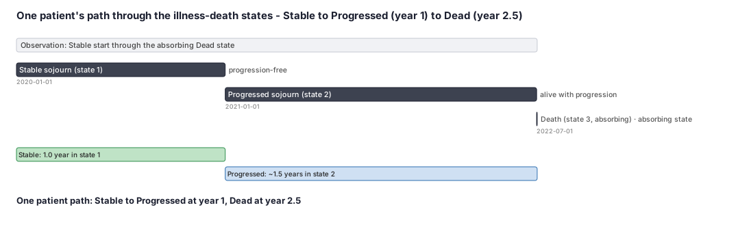
gantt
  title One patient's path through the illness-death states (Stable to Progressed to Dead)
  dateFormat YYYY-MM-DD
  axisFormat %b %Y
  section Stable (state 1)
  Progression-free :crit, s1, 2020-01-01, 366d
  section Progressed (state 2)
  Post-progression alive :active, s2, 2021-01-01, 546d
  section Dead (state 3)
  Death (absorbing) :done, s3, 2022-07-01, 1d
Worked example
Scenario
A 100-patient oncology cohort starts in the Stable state and can move to Progressed or directly to Dead, and from Progressed to Dead - the illness-death model. We observe everyone for two years with no dropout, so the at-risk count in each state is just a headcount. We tabulate who moves at year 1 and year 2, then use the Aalen-Johansen idea (apply each year's transition fractions to the people at risk) to get the probability of occupying each state two years after a Stable start.
Dataset
The at-risk counts and transitions at each event time for the 100-patient illness-death cohort (no dropout) - the table you estimate transition probabilities from.
| event_year | from_state | n_at_risk | n_transitions | to_state |
|---|---|---|---|---|
| 1 | Stable | 100 | 10 | Progressed |
| 1 | Stable | 100 | 5 | Dead |
| 2 | Stable | 85 | 8 | Progressed |
| 2 | Stable | 85 | 4 | Dead |
| 2 | Progressed | 10 | 3 | Dead |
Steps
Result
From a Stable start, the year-2 transition probabilities are 0.73 Stable, 0.15 Progressed, and 0.12 Dead (they sum to 1.00). The 0.15 chance of being alive-with-progression right now is exactly the intermediate-state occupancy a partitioned-survival model cannot read off directly - it falls out of the multi-state structure.
Trade-offs
Runnable example
Nonparametric Aalen-Johansen estimation of the transition-probability matrix P(0, t) from long-format counting-process data, using only numpy and pandas (no specialist package). Required input (one row per at-risk transition episode;
import numpy as np
import pandas as pd

def aalen_johansen(trans: pd.DataFrame, states: list[int], horizon: float):
    """Return P(0, horizon) and the path of P(0, u) at each event time u <= horizon."""
    K = len(states)
    idx = {s: i for i, s in enumerate(states)}
    event_times = sorted(trans.loc[trans["status"] == 1, "t_stop"].unique())

    P = np.eye(K)
    path = []
    for u in event_times:
        if u > horizon:
            break
        dA = np.zeros((K, K))
        for s in states:
            i = idx[s]
            # who is at risk in state s just before time u (unique patients, dedup competing rows)
            at_risk = ((trans["from_state"] == s) &
                       (trans["t_start"] < u) & (trans["t_stop"] >= u))
            n_s = trans.loc[at_risk, "id"].nunique()
            if n_s == 0:
                continue
            fired = trans[(trans["from_state"] == s) &
                          (trans["t_stop"] == u) & (trans["status"] == 1)]
            for to_s, grp in fired.groupby("to_state"):
                dA[i, idx[to_s]] += grp["id"].nunique() / n_s
            dA[i, i] = -dA[i].sum()          # each row of the increment sums to zero
        P = P @ (np.eye(K) + dA)             # product-integral step
        path.append((u, P.copy()))
    return P, path

# P[idx[1]] is then the row of transition probabilities FROM state 1 (Stable) at time 0
# to each state at the horizon - e.g. P[0] = [P(Stable), P(Progressed), P(Dead)].
The mstate workflow: define the transition matrix for an illness-death model, expand wide per-patient data to long counting-process form with msprep, fit transition-specific baseline hazards with a stratified Cox model, and turn the cumulative transition hazards into Aalen-Johansen transition probabilities with...
library(mstate)
library(survival)

# Illness-death model: 1=Stable, 2=Progressed, 3=Dead (3 is absorbing).
tmat <- transMat(x = list(c(2, 3), c(3), c()),
                 names = c("Stable", "Progressed", "Dead"))

# Expand wide data to long: one row per at-risk transition episode (Tstart, Tstop, status, trans).
long <- msprep(time   = c(NA, "pfs_time", "os_time"),
               status = c(NA, "prog",     "death"),
               data   = wide, trans = tmat, keep = c("age", "arm"))
long <- expand.covs(long, covs = c("age", "arm"), append = TRUE)

# Transition-specific baseline hazards: stratify the baseline by transition (clock-forward / Markov).
cox <- coxph(Surv(Tstart, Tstop, status) ~ strata(trans), data = long)

# Cumulative transition hazards -> Aalen-Johansen transition probabilities from each starting state.
msf <- msfit(cox, trans = tmat)
pt  <- probtrans(msf, predt = 0)     # predt=0: P(0, t)
# pt[[1]] = probabilities for patients starting in state 1 (Stable):
#   columns pstate1, pstate2, pstate3 are the occupancy probabilities over time.
head(pt[[1]])

# Semi-Markov (clock-reset) alternative: refit on the per-state sojourn time scale, e.g.
#   coxph(Surv(time, status) ~ strata(trans), data = long)  where `time` = Tstop - Tstart.
Transition-specific hazards via PROC PHREG on counting-process (start, stop) data, stratified by transition. The long table holds one row per at-risk transition episode: long : id, trans, tstart, tstop, status, age, arm where trans codes each allowed move (1: Stable->Progressed, 2: Stable->Dead, 3: Progressed->Dead).
/* 1) Per-transition baseline (Nelson-Aalen) cumulative hazards.
      STRATA trans = a separate baseline hazard per transition; (tstart,tstop) = counting-process input. */
proc phreg data=long;
  strata trans;
  model (tstart, tstop)*status(0) = ;
  baseline out=cumhaz cumhaz=H0;        /* H0 = cumulative hazard for each transition over time */
run;

/* 2) Transition-specific covariate effects: let age and arm act differently by transition. */
proc phreg data=long;
  class trans;
  strata trans;
  model (tstart, tstop)*status(0) = age arm;
run;

/* 3) Assemble Aalen-Johansen transition probabilities from the per-transition hazards in CUMHAZ.
      At each event time u build the increment matrix dA(u) (off-diagonals = hazard jumps d_ss', the
      diagonal set so each row sums to zero), then accumulate the matrix product P = P * (I + dA(u)) in a
      DATA step / IML loop. The result is P(0, t): occupancy probabilities for each starting state over t. */
proc iml;
  use cumhaz; read all var {trans Time H0}; close cumhaz;
  /* ... build dA(u) per distinct Time, multiply forward into P (3x3 here) ... */
quit;
Citations
- [1]Putter H, Fiocco M, Geskus RB. Tutorial in biostatistics: competing risks and multi-state models. Statistics in Medicine. 2007;26(11):2389-2430.
- [2]Andersen PK, Keiding N. Multi-state models for event history analysis. Statistical Methods in Medical Research. 2002;11(2):91-115.