Protopathic Bias and Reverse Causation

In plain language

Protopathic bias happens when a drug is prescribed for the early warning signs of a disease that has not yet been diagnosed — for example, a stomach acid pill given for bloating caused by an undetected stomach cancer. When a researcher later looks at the data, the drug appears to have preceded the disease, creating the illusion that the drug caused it, when in fact the hidden disease caused the prescription. The fix is to ignore drug exposures that occurred in the months immediately before the diagnosis was recorded, a technique called applying a lag window, because those exposures are almost certainly a reaction to early disease symptoms rather than an independent drug use.

What protopathic bias is and how it distorts pharmacoepidemiologic research

Protopathic bias arises when a drug is prescribed not for an independent indication but because of the early, often unrecognized, manifestations of the disease that will later become the outcome variable. The patient already has the disease biologically — cancer cells proliferating, heart failure progressing, a gastric lesion forming — but the clinical record does not yet capture it as a diagnosis. What the prescriber sees is a symptom (pain, epigastric discomfort, dyspnoea, fatigue) and reaches for a drug to palliate it. Months later, when the diagnosis is finally recorded, a researcher examining the database observes a drug fill closely preceding a new diagnosis and, if care is not taken, concludes that the drug caused the disease.

The term was coined by Horwitz and Feinstein (1980), who identified the pattern in case-control studies of drugs and cancer: the drug was not causing the disease, it was responding to the disease's prodrome. The bias is large in magnitude, reliable in direction (it inflates association toward apparent harm or causation), and invisible to standard covariate adjustment. It cannot be corrected by adding confounders to a model, because the disease driving the prescription is the very disease being studied — and it is not (yet) recorded as a covariate.

Classic cases in pharmacoepidemiology

Three drug-outcome pairs illustrate the mechanism across disease categories:

Opioids, antibiotics, and cancer diagnosis. A patient with an unrecognized solid tumor experiences pain from local invasion, weight loss, or bone metastases months before the tumor is found. A clinician prescribes opioids for apparent musculoskeletal pain or antibiotics for apparent infection. When the cancer is eventually diagnosed, the database shows a strong recent-exposure signal. A naive case-control study reads this as "opioid or antibiotic use raises cancer risk" — a near-perfect inversion of causality. The undiagnosed cancer caused the prescription, not the other way around.

PPIs and gastric cancer. Gastric cancer causes dyspepsia, bloating, reflux, and epigastric pain months to years before endoscopy-confirmed diagnosis. These are exactly the symptoms for which proton-pump inhibitors (PPIs) are prescribed. Patients with occult gastric cancer are therefore systematically more likely to have received a recent PPI prescription, producing a spurious positive association. Unadjusted analyses have reported hazard ratios exceeding 2–4; studies applying a 6–12 month lag have seen these estimates collapse toward the null.

Loop diuretics and heart failure. Early, compensated heart failure presents with exertional dyspnoea, ankle swelling, and fluid retention well before echocardiographic confirmation of systolic dysfunction is recorded. Clinicians prescribe loop diuretics for these symptoms. In a database, the patient appears to have received a diuretic before developing heart failure, when in fact the heart failure was already driving the symptoms that prompted the prescription.

Reverse causation and the time-ordering illusion in administrative data

Protopathic bias is a specific, operationally precise instance of the broader category of reverse causation: any situation in which the outcome process causes the exposure, rather than the reverse. Administrative data amplify this problem through a structural artifact — the diagnosis recording date does not equal the biological onset date. Gastric cancer does not begin on the endoscopy report date; heart failure does not begin on the echocardiography date; cancer does not begin on the pathology report date. The diagnostic delay — the gap between biological onset and clinical recognition — can span months to years. During that window the disease is biologically present and symptomatically active, but it is administratively invisible. Any drug exposure measured in that window is contaminated: it looks forward-causal (drug then disease) but is in fact reverse-causal (disease then drug, disease then diagnosis).

Protopathic bias versus confounding by indication: a critical distinction

These two biases are mechanistically distinct, and confusing them leads to wrong remedies. Confounding by indication (channeling) arises when a measured or measurable severity variable simultaneously drives treatment assignment and outcome risk — sicker patients receive more aggressive therapy, so the treated arm reflects disease burden. The path is: recognized severity → treatment and recognized severity → outcome. The disease that causes prescribing is on record as a covariate, and severity-adjustment can reduce the bias. Protopathic bias operates through the unrecognized prodrome of the outcome itself: the very disease being studied, before it is recorded, drives exposure timing. No covariate can correct it because the confounder is the outcome — unobserved. The remedy is temporal, not covariate-based: exclude the exposure that falls within the pre-diagnostic window.

Fixes ranked

[1] Exposure lag/induction windows (primary fix). Exclude all exposures occurring within k months before the index date (diagnosis date for cases; matched date for controls in a case-control study; cohort follow-up entry in a cohort study). The lag k should be motivated by the known prodromal phase of the disease — 6 months for gastric cancer and dyspepsia, 12 months for cancers with longer diagnostic delay. Implement as delayed entry/left truncation on the time axis so person-time and events in the lag are excluded from both numerator and denominator symmetrically across arms. See the exposure-lag-induction-latency-window-rwe entry for operational details.

[2] Latency analyses with varying lag lengths. Report the association at lag = 0, 6, 12, 24, 36 months. A signal that is strongest at lag = 0 and attenuates monotonically with increasing lag is the fingerprint of protopathic bias. A true causal association should be stable or increase at lags consistent with the biological induction period.

[3] Prescription-sequence-symmetry analysis. Compare the sequence of drug prescriptions before versus after the index event. In a true drug-disease causal relationship, the sequences in both directions should be symmetric; protopathic bias predicts that the drug disproportionately precedes the outcome, not follows it. See the prescription-sequence-symmetry entry.

[4] Negative-control outcomes. Select an outcome that the drug cannot biologically cause or protect against. If the association extends to the negative control, residual bias is present. See the negative-control-outcomes-rwe entry.

Pros, cons, and trade-offs

Unlagged (naive) analysis: - Pros: maximal sample size; no a priori lag-length judgment; easy to implement. - Cons: protopathic bias is uncontrolled; estimates can be large multiples of the truth; the bias reliably mimics a causal harmful effect of the drug on the outcome it was prescribed to palliate; downstream clinical or regulatory decisions will be misdirected.

Lagged analysis (primary fix): - Pros: removes or substantially attenuates protopathic bias; the biological motivation for the lag length is transparent, pre-specifiable, and auditable by regulators. - Cons: discards person-time and events, reducing statistical power; the lag length is a judgment call that must be pre-specified and varied in sensitivity analysis; an overly long lag excludes true causal exposure and biases the estimate toward the null. - Trade-off: the lag length should be determined by the known prodromal duration of the disease, not by what makes the association disappear — the latter is post hoc data dredging.

When to use

Apply protopathic-bias assessment and a lagged exposure definition when: (a) the drug being studied is prescribed for symptoms that could be the prodrome of the outcome — analgesics and cancer, acid-suppressive drugs and gastrointestinal malignancy, diuretics and heart failure, antibiotics and sepsis-related diagnoses; (b) the index event (outcome) has a long diagnostic delay (the biological onset substantially precedes the recorded diagnosis date); (c) the study is a case-control design with recent exposure as the primary predictor; (d) a cohort study shows that early-follow-up events drive the association; (e) the study is regulatory-grade and a reviewer has flagged reverse causation as a plausible alternative explanation; (f) any study that will inform drug labeling, regulatory safety communications, or clinical guidelines where a false causal inference would have direct patient harm.

When NOT to use — and when lagging is actively misleading

• Acute, mechanistically immediate outcomes. If the drug causes an acute adverse event —
• Lag chosen post hoc to attenuate a safety signal. A lag length selected after unblinding
• Lag applied to eligibility rather than the time axis. Requiring cases to survive the lag
• As a substitute for active-comparator design. A lag reduces protopathic bias but does not

Interpreting the output

In the worked example (PPI and gastric cancer case-control study), the naive OR is 3.0 and the 6-month-lagged OR is 1.0, using the exact 2x2 counts in the beginner layer.

(1) Formal interpretation. The naive OR = (75 50) / (25 50) = 3.0 is a conditional association estimate from a case-control analysis that counts PPI exposures in the 6 months before the cancer diagnosis date. It does not represent a causal odds ratio. The exposure window is contaminated: 25 of the 75 "exposed" cases were prescribed a PPI during the prodromal phase of their gastric cancer for symptoms attributable to the cancer, not for an independent acid-related condition. After applying a 6-month lag to exclude that window, the cases retain 50 exposed and 50 unexposed patients, identical to controls (50/50), yielding OR = 1.0. The complete attenuation from 3.0 to 1.0 demonstrates that the entire observed association was attributable to the contaminated pre-diagnostic exposure window; the lag removed it entirely. In real data, residual attenuation and CIs spanning 1.0 constitute the evidence against a causal association.

(2) Practical interpretation. If a regulator or payer receives the naive OR of 3.0, they may conclude PPIs cause gastric cancer — a pharmacologically implausible claim that, if acted upon, would withdraw a widely used and effective acid-suppressive drug. The lagged OR of 1.0 tells the true story: PPIs are prescribed because early gastric cancer produces dyspeptic symptoms, not the other way around. Presenting only the naive estimate in a regulatory submission or journal article, without lag analysis, is a methodological failure that directly endangers patients by generating spurious signals and diverting pharmacovigilance attention.

Worked example

Scenario

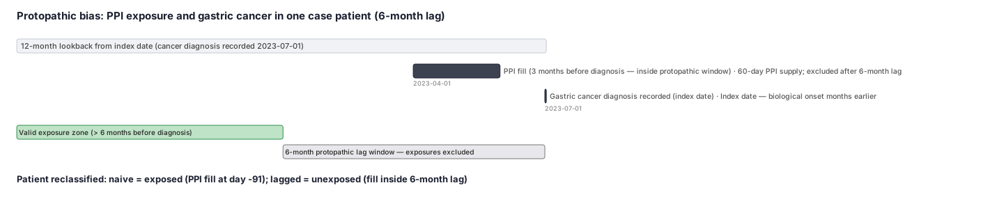
A case-control study asks whether proton-pump inhibitor (PPI) use causes gastric cancer. PPIs are prescribed for dyspepsia, reflux, and epigastric pain — which are also the early symptoms of undiagnosed gastric cancer. The study includes 100 newly diagnosed gastric cancer cases and 100 frequency-matched controls from the same claims database. "Exposed" in the naive analysis means any PPI fill in the 12 months before the diagnosis date (index date). In the lagged analysis, a 6-month lag is applied: PPI fills in the 6 months immediately before the index date are excluded, and only fills from months 7–12 before the index date count as exposure. The 25 cases who had a PPI fill only in the 6-month protopathic window are reclassified as unexposed in the lagged analysis; controls have no early gastric cancer producing prodromal symptoms, so their exposure distribution is unchanged.

Dataset

Two 2x2 tables from the same 100-case, 100-control study. Table A (naive): exposure = any PPI fill in the 12 months before the index date. Table B (6-month lag): exposure = any PPI fill in months 7-12 before the index date only; fills in the 6-month window are excluded.

Steps

• Naive analysis (Table A): cases show 75 exposed and 25 unexposed (row total 75 + 25 = 100); controls show 50 exposed and 50 unexposed (row total 50 + 50 = 100).

• Naive OR = (exposed cases unexposed controls) / (unexposed cases exposed controls) = (75 50) / (25 50) = 3750 / 1250 = 3.0. This 3-fold elevation makes PPIs look strongly associated with gastric cancer.

• But gastric cancer causes dyspepsia, reflux, and epigastric pain months before endoscopic diagnosis. Patients with undetected gastric cancer are prescribed PPIs for those prodromal symptoms, not for an independent acid condition. The disease drives the prescription.

• Applying the 6-month lag: the 25 cases whose only PPI fill was in the 6-month protopathic window are reclassified as unexposed. Cases after lag: 75 - 25 = 50 exposed, 25 + 25 = 50 unexposed. Controls are unchanged because they have no occult gastric cancer generating prodromal symptoms: still 50 exposed and 50 unexposed.

• Lagged OR = (50 50) / (50 50) = 2500 / 2500 = 1.0. After excluding the contaminated pre-diagnostic window, the association disappears entirely.

• The shift from OR = 3.0 at lag = 0 to OR = 1.0 at lag = 6 months is the protopathic-bias fingerprint: the entire observed association resided in the window where disease symptoms were driving prescriptions, not where the drug was acting on the disease.

Result

Table A naive OR = (75 50) / (25 50) = 3.0 (spurious; driven by 25 cases prescribed a PPI for prodromal gastric-cancer symptoms in the 6 months before diagnosis). Table B lagged OR = (50 50) / (50 50) = 1.0 (after excluding the 6-month pre-diagnostic exposure window). The complete attenuation from OR = 3.0 to OR = 1.0 is the fingerprint of protopathic bias.

Timeline Spec

Title

Protopathic bias: PPI exposure and gastric cancer in one case patient (6-month lag)

Window

Start

2022-07-01

End

2023-07-01

Label

12-month lookback from index date (cancer diagnosis recorded 2023-07-01)

Events

• Label

  PPI fill (3 months before diagnosis — inside protopathic window)

  Start

  2023-04-01

  Length Days

  60

  Quantity

  60-day PPI supply; excluded after 6-month lag

• Label

  Gastric cancer diagnosis recorded (index date)

  Start

  2023-07-01

  Length Days

  1

  Quantity

  Index date — biological onset months earlier

Spans

• Kind

  exposed

  Start

  2022-07-01

  End

  2022-12-31

  Label

  Valid exposure zone (> 6 months before diagnosis)

• Kind

  unexposed

  Start

  2023-01-01

  End

  2023-06-30

  Label

  6-month protopathic lag window — exposures excluded

Result

Label

Patient reclassified: naive = exposed (PPI fill at day -91); lagged = unexposed (fill inside 6-month lag)

Runnable example

from math import log, exp, sqrt

# ── 2x2 table helpers ──────────────────────────────────────────────────────────────
def odds_ratio(a, b, c, d):
    """OR = (a*d)/(b*c) where a=exposed cases, b=unexposed cases,
       c=exposed controls, d=unexposed controls."""
    if b == 0 or c == 0:
        raise ValueError("Zero cell prevents OR calculation")
    return (a * d) / (b * c)

def or_95ci(a, b, c, d):
    """95% CI via Woolf log method (valid when all cells > 0)."""
    or_ = odds_ratio(a, b, c, d)
    se_log = sqrt(1/a + 1/b + 1/c + 1/d)
    lo = exp(log(or_) - 1.96 * se_log)
    hi = exp(log(or_) + 1.96 * se_log)
    return or_, lo, hi

# ── Worked-example data ────────────────────────────────────────────────────────────
# Table A: naive (any PPI fill in 12 months before diagnosis)
# a=exposed cases, b=unexposed cases, c=exposed controls, d=unexposed controls
naive  = dict(a=75, b=25, c=50, d=50)

# Table B: 6-month lag applied (fills in 6-month window excluded from cases)
# 25 cases who were exposed only in the lag window -> reclassified as unexposed
lagged = dict(a=50, b=50, c=50, d=50)

print("=== Table A: Naive analysis ===")
or_n, lo_n, hi_n = or_95ci(**naive)
print(f"OR = {or_n:.2f}  95% CI [{lo_n:.2f}, {hi_n:.2f}]")
# Arithmetic: (75 * 50) / (25 * 50) = 3750 / 1250 = 3.0

print("\n=== Table B: 6-month lag applied ===")
or_l, lo_l, hi_l = or_95ci(**lagged)
print(f"OR = {or_l:.2f}  95% CI [{lo_l:.2f}, {hi_l:.2f}]")
# Arithmetic: (50 * 50) / (50 * 50) = 2500 / 2500 = 1.0

# ── Lag-grid sensitivity: vary lag length and reclassify case exposures ──────────
import pandas as pd

def lag_grid_analysis(case_exposures, control_exposures, n_cases, n_controls,
                      index_dates, lag_months_list):
    """
    case_exposures / control_exposures: DataFrames with columns
      [person_id, fill_date, index_date] — one row per fill.
    Returns a DataFrame of OR by lag length for plotting the attenuation pattern.
    """
    results = []
    for lag_m in lag_months_list:
        lag_days = lag_m * 30   # approximate; use relativedelta for production

        # Reclassify: a fill counts only if > lag_days before the index date
        ce = case_exposures.copy()
        ce["days_before"] = (ce["index_date"] - ce["fill_date"]).dt.days
        ce["valid"] = ce["days_before"] > lag_days
        exposed_cases = ce[ce["valid"]].groupby("person_id").size().reset_index()
        a = len(exposed_cases)          # exposed cases after lag
        b = n_cases - a                  # unexposed cases after lag

        co = control_exposures.copy()
        co["days_before"] = (co["index_date"] - co["fill_date"]).dt.days
        co["valid"] = co["days_before"] > lag_days
        exposed_controls = co[co["valid"]].groupby("person_id").size().reset_index()
        c = len(exposed_controls)        # exposed controls
        d = n_controls - c               # unexposed controls

        if b > 0 and c > 0:
            or_val = (a * d) / (b * c)
            results.append({"lag_months": lag_m, "OR": or_val,
                            "a": a, "b": b, "c": c, "d": d})
    return pd.DataFrame(results)

# Protopathic-bias fingerprint: OR attenuates toward 1.0 as lag increases.
# A true causal association stays stable or rises at the induction-period lag.

# ── 2x2 helpers ───────────────────────────────────────────────────────────────────
odds_ratio_woolf <- function(a, b, c, d) {
  # a=exposed cases, b=unexposed cases, c=exposed controls, d=unexposed controls
  # OR = (a*d)/(b*c); 95% CI via Woolf log method
  or <- (a * d) / (b * c)
  se_log <- sqrt(1/a + 1/b + 1/c + 1/d)
  list(OR = or,
       lo = exp(log(or) - 1.96 * se_log),
       hi = exp(log(or) + 1.96 * se_log))
}

# ── Worked-example data ───────────────────────────────────────────────────────────
# Naive: any PPI fill in 12 months before diagnosis date
naive  <- list(a = 75, b = 25, c = 50, d = 50)
# Lagged: 6-month protopathic window excluded; 25 cases reclassified as unexposed
lagged <- list(a = 50, b = 50, c = 50, d = 50)

cat("=== Table A: Naive analysis ===\n")
res_n <- odds_ratio_woolf(naive$a, naive$b, naive$c, naive$d)
cat(sprintf("OR = %.2f  95%% CI [%.2f, %.2f]\n", res_n$OR, res_n$lo, res_n$hi))
# (75 * 50) / (25 * 50) = 3750 / 1250 = 3.0

cat("\n=== Table B: 6-month lag applied ===\n")
res_l <- odds_ratio_woolf(lagged$a, lagged$b, lagged$c, lagged$d)
cat(sprintf("OR = %.2f  95%% CI [%.2f, %.2f]\n", res_l$OR, res_l$lo, res_l$hi))
# (50 * 50) / (50 * 50) = 2500 / 2500 = 1.0

# ── Lag-grid sensitivity (illustrative with synthetic fill-date data) ─────────────
lag_grid <- function(case_fills, ctrl_fills, n_cases, n_ctrls,
                     lag_months_vec = c(0, 6, 12, 24, 36)) {
  # case_fills / ctrl_fills: data.frames with person_id, fill_date, index_date (Date)
  do.call(rbind, lapply(lag_months_vec, function(lag_m) {
    lag_days <- lag_m * 30L

    ce <- case_fills
    ce$days_before <- as.integer(ce$index_date - ce$fill_date)
    ce$valid <- ce$days_before > lag_days
    a <- length(unique(ce$person_id[ce$valid]))
    b <- n_cases - a

    co <- ctrl_fills
    co$days_before <- as.integer(co$index_date - co$fill_date)
    co$valid <- co$days_before > lag_days
    c_ <- length(unique(co$person_id[co$valid]))
    d  <- n_ctrls - c_

    or_val <- if (b > 0 && c_ > 0) (a * d) / (b * c_) else NA_real_
    data.frame(lag_months = lag_m, OR = or_val,
               a = a, b = b, c = c_, d = d)
  }))
}
# Protopathic-bias fingerprint: OR[lag=0] >> OR[lag=6] ~> OR[lag=12] ... approaching 1.
# Plot lag_months vs OR; monotonic decline is the signature.