Relative and Net Survival

In plain language

Relative survival answers the question "how much does a cancer diagnosis reduce a patient's chances of being alive at five years?" without needing to know the exact cause of death -- a piece of information that is often wrong or missing on death certificates. The method compares how many cancer patients actually survived against how many would have been expected to survive based on their age and sex from general-population life tables; the ratio of those two numbers gives net survival, the survival attributable to the cancer alone. A net survival of 0.50 means cancer patients survived at half the rate of comparable people in the general population, with the gap blamed on the cancer and its treatment rather than background diseases like heart attacks or strokes.

The cancer-registry problem that motivates relative survival

In most cancer registries, the death certificate records a cause of death -- but those entries are notoriously unreliable. A patient with stage-IV colon cancer who dies of myocardial infarction may be coded as a cancer death; a patient dying of uncontrolled metastatic disease may be certified as dying of sepsis. Misclassification is differential by cancer site, age, race/ethnicity, and data period. In Medicare claims and other administrative sources the problem is worse still: the only cause-of-death signal is the ICD code on the discharge claim or the enrollment death-file entry, not a reviewed death certificate. The practical consequence is that cause-specific survival analysis requires knowing why a patient died, and that knowledge is often unavailable, partial, or systematically wrong in population-based registry data. Relative survival bypasses the problem entirely: it never asks why a patient died, only whether the rate at which they died exceeded what was expected from the general population of the same age, sex, and calendar year.

The estimand: net survival

Net survival is the survival probability in a conceptual world where the cancer is the only possible cause of death -- all background mortality has been removed by assumption. It is not the observed all-cause survival (which includes deaths from heart disease, stroke, and accidents unrelated to the cancer), and it is not cause-specific survival (which requires reliable cause-of-death coding). Net survival is the quantity that SEER data products, CONCORD, and EUROCARE comparisons report, and it is the international standard for population-based cancer surveillance. The Pohar Perme estimator (2012) is the nonparametric estimator of net survival that is unbiased under the independence assumption: a patient's expected general-population survival is independent of their actual cancer prognosis given age, sex, and calendar year. This is the current recommendation of the International Agency for Research on Cancer.

The relative survival ratio: observed divided by expected

Relative survival is computed as:

relative_survival = observed_survival / expected_survival

where observed_survival is the all-cause Kaplan-Meier survival probability from the cancer cohort, and expected_survival is the survival probability that the cohort would have experienced if they had the same all-cause mortality as the general population matched on age, sex, and calendar year -- obtained from population life tables. A relative survival of 0.50 at five years means the cancer cohort survived at 50% of the rate that a comparable general-population group would have survived. Note: the 0.50 is a ratio, not a percentage-point deficit — the absolute deficit in this example is 40 percentage points (observed 0.40 minus expected 0.80 = −0.40). Relative survival above 1.0 is possible (a healthy-worker effect or a population selected for low baseline mortality) but requires careful interpretation. Statistical cure in the net survival framework is indicated when the excess hazard returns to zero and the relative survival curve plateaus — it stops declining and stabilises at a fixed value that equals the proportion of the cohort effectively cured. This plateau is generally below 1.0 unless all patients are eventually cured; relative survival does not in general approach 1.0 as follow-up lengthens.

Pohar Perme versus Ederer I, Ederer II, and Hakulinen: why the estimator matters

Older methods -- Ederer I (1961), Ederer II (1961), and Hakulinen (1982) -- estimated relative survival using different constructions of expected survival in the denominator. All three are biased when the age distribution within the cohort is informative -- which it almost always is in cancer data, because older patients both have worse cancer prognosis and worse expected general-population survival. The bias is upward: older patients accumulate deaths quickly and exit the risk set early, so later survival estimates come from the younger (better-prognosis) survivors; the expected-survival denominator is incorrectly handled, and net survival is over-estimated. Pohar Perme (2012) corrected this by inverse probability weighting: at each event time, each patient is up-weighted by the inverse of their expected general-population survival, amplifying the contribution of older patients whose expected mortality is high and whose net survival would otherwise be under-counted. In practice the Pohar Perme estimate is lower than Ederer II for older, higher-mortality cancer cohorts -- which is the correct direction; the earlier estimators were optimistically biased. Use Pohar Perme for all new analyses; revisit Ederer II only when replicating historical literature.

Life-table choice: national, regional, SES-specific, and the US claims-data caveat

The expected-survival denominator comes from a population life table stratified by age, sex, and calendar year. In most countries the national life table is the default comparator, and it is required for international comparisons. However:

• Regional or socioeconomic-stratum-specific tables give more accurate comparators when the
• In the United States, commercially insured populations have substantially lower all-cause
• Medicare populations are closer to the national elderly life table, but the dual-eligible

Age-standardization for comparisons across registries and time periods

Comparing relative survival across cancer registries, time periods, or countries requires age-standardization, because different populations diagnose cancer patients at different age distributions. The International Cancer Survival Standard (ICSS) provides three weight sets for different cancer sites. The age-standardized relative survival is a weighted average of age-stratum-specific relative survival estimates using the ICSS weights (Corazziari et al. 2004) -- one line of arithmetic applied after stratum-specific estimation.

Excess hazard regression

When covariates must be modeled, the relative-survival framework uses excess hazard regression. The total observed hazard in the cancer cohort is decomposed as:

total_hazard = excess_hazard + expected_hazard

where expected_hazard is read from the life table at each patient's age/sex/year, and excess_hazard is the cancer-attributable component to be modeled. The excess hazard is modeled as a function of covariates (cancer stage, grade, treatment, socioeconomic status) using Poisson regression with an offset for the expected hazard (Dickman et al. 2004). Regression coefficients are excess hazard ratios: the multiplicative change in cancer-attributable mortality associated with a one-unit change in the covariate. Excess hazard regression is the relative-survival analogue of Cox regression for cause-specific survival.

Route to relative survival cure models

When the excess hazard returns to zero at finite follow-up -- the cohort's survival converges to the matched general-population life table -- there is statistical evidence of cure. Relative survival cure models partition the cohort into a cured fraction (those whose excess hazard has reached zero) and an uncured fraction still experiencing excess mortality. The cured fraction's survival thereafter follows the general-population life table. This is one of the primary input pathways for mixture-cure models in cancer registry settings; see the cure-models-mixture-cure entry for the full cure-model framework. Relative survival provides the necessary input when cause-of-death data are unavailable.

Pros, cons, and trade-offs

Relative / net survival versus cause-specific survival (when cause-of-death data exist): - Pros: Requires no cause-of-death coding at all; immune to misclassification of cause; directly comparable across registries with varying certification quality; the established standard for population-based cancer surveillance; estimable from any population with a matching life table. - Cons: Requires a matching population life table that accurately represents the background mortality of the study cohort; depends on the independence assumption (discussed above); cannot separate deaths caused by the cancer from deaths caused by cancer treatment toxicity (both are "excess" mortality); relative survival can exceed 1.0 in selected populations, which is numerically unintuitive; the Pohar Perme estimator has slightly higher variance than the simpler Ederer II at small sample sizes. - When to prefer: Population-based registry studies, SEER, EUROCARE, national cancer-plan evaluations, and any setting where cause-of-death coding is unreliable, missing, or differentially misclassified across comparison groups.

National versus population-specific life tables: - Pros of national tables: Universally available; standard for international comparisons; simple to implement. - Cons: Can over- or under-state expected mortality in non-representative cohorts (insured, rural, SES extreme). For US commercial-claims analyses, the national table overstates expected mortality rates, which deflates the expected survival denominator and thereby inflates the relative survival estimate, making the cancer appear less lethal than it is in that insured population. - When to prefer: National tables for SEER and registry work; population-specific or insured-cohort life tables for claims-based analyses when available, or at minimum as a sensitivity analysis.

When to use

Use relative and net survival when: the primary analysis is population-based cancer survival using registry data where cause-of-death is unreliable or unavailable; when the deliverable is a net survival probability for time-trend comparison or cross-registry benchmarking where consistency of cause-of-death coding cannot be assumed; when a population life table matched on age, sex, and calendar year is available and the independence assumption is defensible; when excess hazard regression is the preferred modeling framework for covariate adjustment in a registry-based cancer survival study; or when a cure-model analysis is planned and cause-of-death data are not available.

When NOT to use

• Non-fatal outcomes: Relative survival is a survival-only framework. For outcomes such as
• *When reliable cause-of-death data are available and a cause-specific estimand is the
• When the independence assumption is materially violated: If the cancer shares strong risk
• Do not apply to US commercial-claims data without a population-appropriate life table:

Interpreting the output

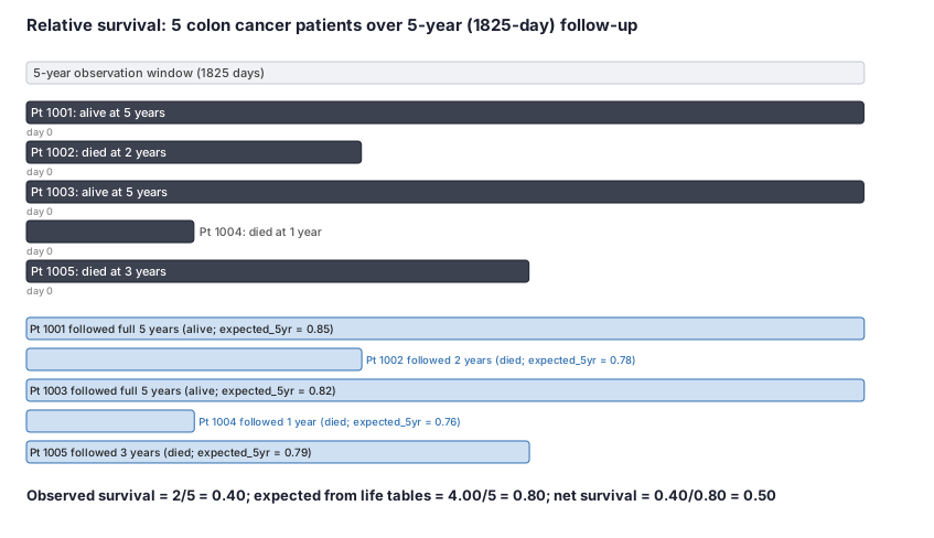
From the worked example: a colon cancer cohort of 5 patients followed 5 years. Observed all-cause survival at 5 years = 0.40 (2 of 5 patients alive at 5 years). Mean expected 5-year survival from matched life tables (age/sex/calendar year) = 0.80. Net (relative) survival = 0.40 / 0.80 = 0.50.

(1) Formal interpretation. The relative survival of 0.50 is an estimate of net survival computed here as a simple Ederer-style observed/mean-expected ratio — the worked example uses this transparent arithmetic to illustrate the concept. The Pohar Perme estimator applies inverse-probability weighting at each event time (upweighting older patients whose background mortality is higher) and gives a different, unbiased estimate; it should be used in any real analysis. Under the independence assumption that each patient's expected general-population survival is independent of their actual cancer prognosis conditional on age, sex, and calendar year, the Pohar Perme estimator is consistent for net survival. Relative survival is a ratio of two survival probabilities, not itself a bounded probability; it can exceed 1.0 in populations with below-national-average background mortality. A value of 0.50 means the cancer cohort's observed all-cause survival is 50% of what the same-age, same-sex general population would have experienced -- with the remaining deficit attributed to the excess mortality from colon cancer and its treatment.

(2) Practical interpretation. The relative survival of 0.50 is a ratio: the cohort survived at half the rate of the matched general population (0.40 vs. 0.80). The absolute deficit is 0.80 − 0.40 = 0.40 — approximately 40 fewer would be alive per 100 newly diagnosed patients at 5 years compared with similarly aged people in the general population who did not receive a cancer diagnosis. The 0.50 itself is not a 50-percentage-point deficit; confusing the ratio with the absolute gap is a common communication error. This is the quantity reported in international cancer-survival comparisons (CONCORD, EUROCARE) and in SEER publications; it is interpretable across time periods and registries regardless of differences in cause-of-death certification quality. For clinical communication, emphasize that it represents the survival experience attributable to the cancer diagnosis itself, net of the background mortality that those patients would have experienced regardless of the cancer.

Worked example

Scenario

A state cancer registry tracks 5 patients newly diagnosed with colon cancer in 2018, all followed for exactly 5 years. For each patient, the registry also records their expected 5-year survival probability, looked up from the US national life table matched on their age at diagnosis, sex, and calendar year. We want to estimate the 5-year net survival for this cancer -- the survival attributable to the colon cancer itself, independent of background mortality. Two patients are still alive at 5 years; three died during follow-up. Because death certificates in this registry are not reliably coded for cancer vs non-cancer cause, we use relative survival rather than cause-specific survival.

Dataset

One row per patient: follow-up outcome at 5 years and life-table expected 5-year survival. Expected survival is the probability the general population (matched on age/sex/year) would survive 5 years, read from the US national life table.

Steps

• Step 1 -- Count patients alive at 5 years: patients 1001 and 1003 survived all 1825 days. Observed 5-year survival: 2 / 5 = 0.40.

• Step 2 -- Compute mean expected 5-year survival from life tables: sum of expected_5yr = 0.85 + 0.78 + 0.82 + 0.76 + 0.79 = 4.00; mean expected survival = 4.00 / 5 = 0.80. This is the survival the age/sex/year-matched general population would have experienced.

• Step 3 -- Compute relative (net) survival: 0.40 / 0.80 = 0.5. This is the net survival estimate: for every person in the general population who survived 5 years, only 0.50 of the cancer patients survived, with the deficit attributed to the colon cancer.

• Step 4 -- Interpretation: a net survival of 0.5 means the colon cancer cohort had 50% of the 5-year survival probability that their age/sex/year-matched general-population counterparts had. The 40% observed survival minus the 80% expected survival yields the 40-percentage-point gap attributable to the cancer and its treatment.

Result

Observed 5-year survival = 2 / 5 = 0.40. Mean expected 5-year survival from life tables = 4.00 / 5 = 0.80. Relative (net) 5-year survival = 0.40 / 0.80 = 0.50. Net survival of 0.50 means this cancer cohort survived at 50% the rate of the age/sex-matched general population; the 50% deficit is attributed to the colon cancer and its treatment, net of background mortality.

Timeline Spec

Title

Relative survival: 5 colon cancer patients over 5-year (1825-day) follow-up

Window

End Day

1825

Label

5-year observation window (1825 days)

Events

• Label

  Pt 1001: alive at 5 years

  End Day

  1825

  Marker

  Alive at day 1825 (5 years)

• Label

  Pt 1002: died at 2 years

  End Day

  730

  Marker

  Death at day 730

• Label

  Pt 1003: alive at 5 years

  End Day

  1825

  Marker

  Alive at day 1825 (5 years)

• Label

  Pt 1004: died at 1 year

  End Day

  365

  Marker

  Death at day 365

• Label

  Pt 1005: died at 3 years

  End Day

  1095

  Marker

  Death at day 1095

Spans

• Kind

  followup

  End Day

  1825

  Label

  Pt 1001 followed full 5 years (alive; expected_5yr = 0.85)

• Kind

  followup

  End Day

  730

  Label

  Pt 1002 followed 2 years (died; expected_5yr = 0.78)

• Kind

  followup

  End Day

  1825

  Label

  Pt 1003 followed full 5 years (alive; expected_5yr = 0.82)

• Kind

  followup

  End Day

  365

  Label

  Pt 1004 followed 1 year (died; expected_5yr = 0.76)

• Kind

  followup

  End Day

  1095

  Label

  Pt 1005 followed 3 years (died; expected_5yr = 0.79)

Result

Label

Observed survival = 2/5 = 0.40; expected from life tables = 4.00/5 = 0.80; net survival = 0.40/0.80 = 0.50

Observed Survival

0.4

Expected Survival

0.8

Net Survival

0.5

Caption

Each horizontal bar shows one patient's follow-up from Day 0. Patients 1001 and 1003 (green) survived the full 1825 days; patients 1002, 1004, and 1005 (red) died before 5 years. The observed 5-year survival of 0.40 (2 of 5 alive) is divided by the mean expected survival of 0.80 from age/sex/year-matched life tables to yield net survival = 0.50. Without cause-of-death coding, this relative-survival calculation isolates the cancer's contribution to excess mortality.

Alt Text

Five horizontal patient-timeline bars from Day 0 to their end. Patients 1001 and 1003 extend the full 1825 days (5 years) with alive markers; patients 1002, 1004, and 1005 end at days 730, 365, and 1095 respectively with death markers. An annotation shows observed 5-year survival = 0.40, expected from life tables = 0.80, and net survival = 0.50.

Runnable example

import pandas as pd
from lifelines import KaplanMeierFitter

# ── Worked-example cohort (5 colon cancer patients) ──
data = pd.DataFrame({
    "person_id":    [1001,  1002,  1003,  1004,  1005],
    "fu_days":      [1825,   730,  1825,   365,  1095],
    "event":        [   0,     1,     0,     1,     1],   # 0=alive, 1=dead (all-cause)
    "expected_5yr": [0.85,  0.78,  0.82,  0.76,  0.79],  # from national life table
})

HORIZON_DAYS = 1825  # 5 years

# ── 1. Observed all-cause survival at 5 years (Kaplan-Meier) ──
kmf = KaplanMeierFitter()
kmf.fit(data["fu_days"], event_observed=data["event"])
observed_surv = float(kmf.predict(HORIZON_DAYS))
print(f"Observed 5-year survival (KM):      {observed_surv:.4f}")

# ── 2. Mean expected 5-year survival from the life table ──
expected_surv = data["expected_5yr"].mean()
print(f"Mean expected 5-year survival (LT): {expected_surv:.4f}")

# ── 3. Relative (net) survival = observed / expected ──
# NOTE: This simple ratio is the intuitive definition. The Pohar Perme estimator applies
# inverse-probability weights at each event time to remove the age-structure bias; the
# ratio below agrees with the worked example (0.40 / 0.80 = 0.50) but does not implement
# the full weighting. Use relsurv in R for production Pohar Perme estimation.
relative_surv = observed_surv / expected_surv
print(f"Relative (net) 5-year survival:     {relative_surv:.4f}")
print()
print("Verify: 2 alive / 5 total = 0.40 observed; "
      "sum expected = 4.00, mean = 0.80; ratio = 0.40 / 0.80 = 0.50")

# ── 4. Excess hazard (approximate, for illustration) ──
# For a single time horizon, excess cumulative hazard = -ln(rel_surv).
import math
excess_cum_haz = -math.log(relative_surv) if relative_surv > 0 else float("inf")
print(f"Approximate 5-year cumulative excess hazard: {excess_cum_haz:.4f}")
print("For full excess hazard regression, use relsurv::excess() or popEpi::relpoisreg in R.")

library(relsurv)
library(survival)

# ── Minimal worked-example dataset (5 patients, matches the Python/beginner example) ──
d <- data.frame(
  fu_time   = c(1825, 730, 1825, 365, 1095),  # days of follow-up
  event     = c(   0,   1,    0,   1,    1),   # all-cause death (0=alive, 1=dead)
  age_dx    = c(  62,  71,   58,  75,  68),    # age at diagnosis (illustrative)
  sex       = c(   2,   1,    2,   1,   1),    # 1=male, 2=female (ratetable convention)
  diag_year = c(2000, 2000, 2000, 2000, 2000)  # calendar year of diagnosis
# NOTE: slopop covers US 1940-2004; use diag_year within that range.
# For 2018 or later diagnoses, use a current life table (e.g., from the Human
# Mortality Database or survexp.us from the survival package, extended to recent years).
)
# Build the ratetable entry date (first day of year of diagnosis)
d$entry_date <- as.Date(paste0(d$diag_year, "-01-01"))

## 1. Pohar Perme nonparametric net survival curve.
# ratetable() links each patient to the US national life table (slopop).
# fu_time must be in days; ratetable uses age-in-years, sex, and a calendar Date.
rs <- rs.surv(
  Surv(fu_time, event) ~ 1,
  rmap   = list(age  = age_dx * 365.25,   # relsurv expects age in days
                sex  = sex,
                year = entry_date),
  data   = d,
  ratetable = slopop,                      # US national life table (1940-2004 coverage)
  method = "pohar-perme"                   # IARC-recommended; unbiased for net survival
)
print(summary(rs, times = 1825))            # 5-year net survival estimate + 95% CI

## 2. Net survival by a covariate (e.g., stage group) using rs.surv with a strata term.
# Extend d with a stage variable for illustration:
# rs_stage <- rs.surv(Surv(fu_time, event) ~ stage_group, rmap = list(...), ...)
# Age-standardize across ICSS weight strata after computing stratum-specific estimates.

## 3. Excess hazard regression: Poisson model for covariate adjustment.
# Creates split person-time records (one row per interval) with the expected hazard as offset.
# The excess() function returns an excess hazard ratio for each covariate.
# Illustrative with stage_group (factor); replace with real covariates.
d$stage_group <- factor(c("III", "II", "III", "IV", "II"))  # illustrative only
ex_model <- excess(
  Surv(fu_time, event) ~ stage_group,
  rmap      = list(age = age_dx * 365.25, sex = sex, year = entry_date),
  data      = d,
  ratetable = slopop,
  method    = "glm"   # Poisson excess hazard (Dickman et al. 2004)
)
summary(ex_model)   # excess hazard ratios (EHR) per covariate level