Kaplan-Meier Estimator

In plain language

The Kaplan-Meier curve is a way to draw the fraction of patients who have not yet had a specific event (such as hospitalization or death) at each point in time, using data from a group where some patients leave the study early without having the event (called censored patients). It works by computing, at each moment when an event occurs, the fraction of the patients still being observed who had the event, then multiplying those fractions together progressively to get an ever-updating "survival" probability. The curve's most practical output is the median survival time — the day by which half the group has had the event — along with a table showing how many patients were still being counted at each point, which warns you when the estimate is based on only a few remaining patients and should not be trusted too precisely.

Product-limit construction: risk sets and conditional survival at each event time

The Kaplan-Meier estimator builds the survival curve one event at a time. Let t_1 < t_2 < ... < t_k denote the distinct times at which events occur (ties are handled by treating the event and any same-day censorings together). At each event time t_j, define n_j as the number of subjects still in the risk set (not yet had the event, not yet censored before t_j) and d_j as the number of events that occur at exactly t_j. The conditional probability of surviving past t_j, given survival to t_j, is (n_j - d_j) / n_j. The Kaplan-Meier estimate at time t is the cumulative product of all such conditional probabilities for event times up to and including t:

S_KM(t) = product over all j with t_j <= t of ((n_j - d_j) / n_j)

This product-limit formula is what Kaplan and Meier (1958) introduced. Its power comes from updating the risk set after every event: subjects who are censored between consecutive event times exit the risk set before the next event, so the denominator shrinks and each subsequent conditional probability uses only those still observed. Censored subjects contribute their observed follow-up time to every risk set they are part of before exit; they do not contribute to the event count d_j. The resulting step function drops only at observed event times and is flat between them, making it easy to read off the probability of being event-free at any given time.

Median survival time and quantiles from the curve

The KM median survival time is the smallest t at which the curve drops to or below 0.5 (i.e., S_KM(t) ≤ 0.5). If the curve never reaches 0.5 within the observation window — because too many subjects are censored before enough events accumulate — the median is undefined or reported as ">last event time." Similarly, the p-th quantile (e.g., the 25th or 75th percentile of the event-time distribution) is read as the smallest t where S_KM(t) ≤ (1 - p). These quantiles are robust to the non-normal shape typical of time-to-event data in RWE and are the primary summaries reported alongside KM curves in publications and regulatory submissions.

Greenwood variance and confidence interval bands

The variance of the KM estimator at time t is estimated by the Greenwood formula:

Var[S_KM(t)] = S_KM(t)^2 sum over j with t_j <= t of (d_j / (n_j (n_j - d_j)))

Pointwise 95% confidence intervals are typically constructed on the log or log-log scale (so the CI is guaranteed to stay in [0, 1]) and then back-transformed. The Hall-Wellner and equal-precision (EP) bands, used in SAS PROC LIFETEST and R survfit(), are simultaneous bands that cover the entire curve at a nominal confidence level. The CI widens as the risk set shrinks — notably at the right tail of the curve, where few subjects remain after heavy censoring. A KM curve that drops sharply in its final steps with extremely wide CI bands signals that the tail estimate is unreliable, a near-universal occurrence in claims data where late follow-up is dominated by the few persistent enrollees.

Assumptions: non-informative censoring

The foundational assumption is that censoring is non-informative (equivalently, independent): at any event time t, subjects censored at t have the same future event hazard as those still under observation. When this holds, the risk-set calculation is valid — the censored subjects who exit are a random draw from those still at risk, not a systematically sicker or healthier subset. In real-world insurance claims, this assumption is threatened by health-correlated disenrollment: patients who lose coverage due to job loss tied to worsening disease, or who transition to Medicare Advantage plans because of escalating care needs, leave the observable risk set at elevated risk. The direction of the bias is typically optimistic — the remaining, observable subjects are healthier than those who left — and the KM curve overstates survival probability. See the censoring-mechanisms-rwe entry for a full taxonomy of censoring types and when the non-informative assumption fails.

Number-at-risk tables: mandatory reporting

A KM curve without a number-at-risk table is incomplete. The number at risk at each displayed time point (typically at regular intervals below the x-axis) tells the reader how many subjects were still contributing to the estimate at that moment. A curve that appears smooth and well-estimated at month 24 in a study that enrolled 10,000 patients may be based on only 200 at-risk individuals if enrollment was staggered and administrative censoring was common. Regulatory guidance from the FDA and EMA, as well as methodological standards from Pocock et al. (2002), treat the at-risk table as non-negotiable. Both ggsurvfit (R) and PROC LIFETEST (SAS) produce at-risk rows natively.

KM versus 1 minus KM and the competing-risks overestimation trap

A common mistake is reporting 1 - S_KM(t) as the cumulative incidence of the event when a competing risk (most often death) is present and non-negligible. Treating death as censoring when the event of interest is a non-fatal outcome (readmission, stroke, medication failure) assumes the censored-dead patients remain at risk of the non-fatal outcome — which is impossible. The 1 - KM curve therefore overestimates cumulative incidence in a real population where mortality removes subjects permanently, and the overestimation is differential when mortality rates differ by treatment arm. When competing risks are present, the correct descriptive estimator is the Aalen-Johansen cumulative incidence function, which treats competing events as distinct exit types rather than censoring. See the competing-risks-cause-specific-fine-gray-rwe and cumulative-incidence-risk-rwe entries for full treatment.

No covariate adjustment: KM is descriptive

The KM estimator makes no distributional assumption and accepts no covariates. It describes observed (possibly confounded) survival in the data as delivered. If two arms differ in baseline age, comorbidity, or frailty, the KM curves absorb those imbalances — the estimator will not adjust for them. Covariate-adjusted survival curves require either (a) Cox proportional hazards regression with the baseline covariates as predictors and the curve predicted at representative covariate values, or (b) standardization (direct adjustment) over the covariate distribution of a reference population. These adjusted curves carry the proportional-hazards or model-specification assumption that KM avoids, so reporting the unadjusted KM alongside adjusted estimates is standard practice for transparency.

Claims-specific considerations

In commercial insurance claims, the dominant censoring mechanism is plan disenrollment, which is typically health-correlated (see above). The risk set at the tail of the KM curve in a 12-month or 24-month study is often small — fewer than 5 to 10 percent of the original cohort — because enrollment gaps and plan switches remove subjects over time. KM estimates at the tail based on fewer than 10 to 20 subjects at risk are unstable: a single event can drop the curve by 5 to 10 percentage points, and the CI bands expand dramatically. The convention in regulatory pharmacoepidemiology is to truncate the displayed KM curve at the time when fewer than 10 subjects remain at risk, or to report only up to the time when 80 percent of the cohort has been censored. HEOR reports to payers should follow this convention and include the at-risk counts explicitly.

Pros, cons, and trade-offs

Pros of the Kaplan-Meier estimator: - Fully nonparametric — makes no assumption about the shape of the underlying event-time distribution; valid for exponential, Weibull, log-normal, and unknown distributions alike. - Accommodates censoring rigorously through the risk-set mechanism, provided the non-informative censoring assumption holds. - Produces a visual curve that communicates survival probability intuitively to clinical and payer audiences. - The log-rank test is the natural companion for group comparisons (see log-rank-test).

Cons: - Purely descriptive: no covariate adjustment, no causal inference without additional assumptions and methods. - The non-informative censoring assumption is often violated in insurance claims, biasing the curve optimistically when the sickest patients disenroll earliest. - Tail instability: small risk sets at late time points yield wide CI bands and unstable point estimates. - Incorrectly applied to competing-risk settings (treating death as censoring) produces upward-biased cumulative incidence estimates. - The KM curve and median survival are not directly usable in cost-effectiveness models that require hazard rates or parametric distributions; parametric fitting or RMST is needed for extrapolation.

When to use

Use the Kaplan-Meier estimator as the primary descriptive tool whenever the outcome is a time-to-event endpoint and the research question is "what fraction of the population remained event-free by time t?" It is appropriate for: - Comparative effectiveness and safety studies where unadjusted group-level survival curves are needed as a starting point or visual summary. - Regulatory submissions to FDA and EMA, where KM curves with at-risk tables are a standard component of the clinical and safety sections. - Phase II or pilot studies where the non-parametric approach avoids parametric misspecification in small samples. - Any setting where the log-rank test will be used, since both share the same risk-set framework and the KM curve is the natural visual companion.

When NOT to use — and when this is actively misleading

Do not use the Kaplan-Meier 1 - S_KM(t) curve as the cumulative incidence when a competing event is non-negligible — typically death in any study of older patients or serious chronic conditions. This is the most consequential misapplication in RWE. The overestimation of absolute risk can be clinically and policy-relevant in magnitude (often 1 to 3 percentage points at 12 months in elderly cohorts), and the bias is differential by arm when competing mortality differs.

Do not use KM as the primary analysis when group imbalance must be controlled: the estimator has no mechanism for covariate adjustment. In an observational study without adequate matching or weighting, the KM curves reflect a confounded comparison, and reporting them as if they estimate a causal contrast is misleading. Use Cox regression or standardized survival curves for adjusted inference, and report KM as descriptive background.

Do not extend the curve beyond the time when the risk set becomes small (fewer than 10 to 20 subjects). The curve is arithmetically valid but practically useless in that region, and presenting a smooth-looking KM tail based on two or three subjects at risk misleads the audience about the precision of the estimate.

Do not use KM for long-horizon extrapolation (e.g., lifetime survival for a cost-utility model). The curve is anchored to observed follow-up; extrapolating requires parametric survival models fitted to the observed data and validated against external sources.

Interpreting the output

In the 10-patient worked example, the KM curve estimates S(10) = 0.9, S(30) = 0.7875, S(50) = 0.63, and S(70) = 0.4725. The median survival time is 70 days.

Formal interpretation: the KM survival probability of 0.4725 at day 70 is the estimated probability of remaining event-free through day 70, under the assumption that the six censored subjects were censored non-informatically (i.e., their residual event risk was the same as those who remained under observation at each event time). The estimate is a product of four conditional probabilities — one at each observed event time — and it is the maximum-likelihood estimator of the event-time distribution in the nonparametric family. The stated median of 70 days is the smallest observed time at which the estimated event-free probability drops to or below 0.5. After day 70, only three subjects remain in the risk set (all censored); the curve stays at 0.4725 and the CI expands, signaling that the tail is no longer reliably estimated.

Practical interpretation: approximately half of patients in this cohort would be expected to have had the event by day 70. However, the estimate is based on 10 patients and 4 events; the confidence interval around the median is wide and the result should be treated as a pilot estimate, not a definitive survival probability. In a real claims analysis with thousands of patients, the same calculation applies mechanically but the risk-set stability and the plausibility of the non-informative censoring assumption both require explicit documentation and, in regulatory submissions, a sensitivity analysis.

Worked example

Scenario

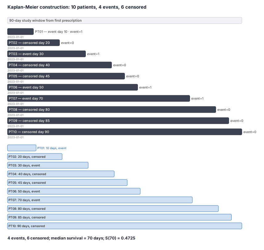
Ten patients newly prescribed a diabetes medication are followed from their first prescription (day 0) to see whether they are hospitalized for a hypoglycemia-related event. Some patients experience the event; others drop their insurance plan or reach the end of the 90-day study window without any event (censored). The analyst builds the Kaplan-Meier survival curve step by step to estimate what fraction of patients remain event-free at each event time, and reads off the median time to first hospitalization.

Dataset

One row per patient. Event = 1 means a hospitalization occurred; event = 0 means the patient was censored (left observation without the event). Follow-up days is the number of days from first prescription to event or censoring.

Steps

• Sort all follow-up times. Distinct event times (where event = 1 occurs) are days 10, 30, 50, and 70. Censoring times (days 20, 40, 45, 80, 85, 90) shrink the risk set before the next event but do not trigger a step-down in the curve.

• Day 10: All 10 patients are in the risk set. One event occurs (PT01). Conditional survival = (10-1)/10 = 9/10 = 0.9. S(10) = 9/10 = 0.9.

• Between days 10 and 30: PT02 is censored at day 20 and exits the risk set. Risk set at day 30 = 10 - 1 event (day 10) - 1 censored (day 20) = 8 patients.

• Day 30: 8 patients in the risk set. One event occurs (PT03). Conditional survival = (8-1)/8 = 7/8. S(30) = 0.9 * 7/8 = 0.7875.

• Between days 30 and 50: PT04 censored at day 40, PT05 censored at day 45. Risk set at day 50 = 8 - 1 event (day 30) - 2 censored (days 40 and 45) = 5 patients.

• Day 50: 5 patients in the risk set. One event occurs (PT06). Conditional survival = (5-1)/5 = 4/5. S(50) = 0.7875 * 4/5 = 0.63.

• Between days 50 and 70: no censorings. Risk set at day 70 = 5 - 1 event (day 50) = 4 patients.

• Day 70: 4 patients in the risk set. One event occurs (PT07). Conditional survival = (4-1)/4 = 3/4. S(70) = 0.63 * 3/4 = 0.4725.

• After day 70: PT08 censored at day 80, PT09 at day 85, PT10 at day 90. No further events occur. The curve stays flat at S = 0.4725. Since S(70) = 0.4725 is the first value at or below 0.5, the median survival time is 70 days.

Result

KM survival probabilities at each event time: S(10) = 9/10 = 0.9; S(30) = 0.9 7/8 = 0.7875; S(50) = 0.7875 4/5 = 0.63; S(70) = 0.63 * 3/4 = 0.4725. Median survival = 70 days (first time S(t) drops to or below 0.5). Four events, six censored. After day 70 only three patients remain in the risk set; the tail estimate is unreliable.

Timeline Spec

Title

Kaplan-Meier construction: 10 patients, 4 events, 6 censored

Window

Start

2023-01-01

End

2023-03-31

Label

90-day study window from first prescription

Events

• Label

  PT01 — event day 10

  Start

  2023-01-01

  Length Days

  10

  Quantity

  event=1

• Label

  PT02 — censored day 20

  Start

  2023-01-01

  Length Days

  20

  Quantity

  event=0

• Label

  PT03 — event day 30

  Start

  2023-01-01

  Length Days

  30

  Quantity

  event=1

• Label

  PT04 — censored day 40

  Start

  2023-01-01

  Length Days

  40

  Quantity

  event=0

• Label

  PT05 — censored day 45

  Start

  2023-01-01

  Length Days

  45

  Quantity

  event=0

• Label

  PT06 — event day 50

  Start

  2023-01-01

  Length Days

  50

  Quantity

  event=1

• Label

  PT07 — event day 70

  Start

  2023-01-01

  Length Days

  70

  Quantity

  event=1

• Label

  PT08 — censored day 80

  Start

  2023-01-01

  Length Days

  80

  Quantity

  event=0

• Label

  PT09 — censored day 85

  Start

  2023-01-01

  Length Days

  85

  Quantity

  event=0

• Label

  PT10 — censored day 90

  Start

  2023-01-01

  Length Days

  90

  Quantity

  event=0

Spans

• Kind

  followup

  Start

  2023-01-01

  End

  2023-01-11

  Label

  PT01: 10 days, event

• Kind

  followup

  Start

  2023-01-01

  End

  2023-01-21

  Label

  PT02: 20 days, censored

• Kind

  followup

  Start

  2023-01-01

  End

  2023-01-31

  Label

  PT03: 30 days, event

• Kind

  followup

  Start

  2023-01-01

  End

  2023-02-10

  Label

  PT04: 40 days, censored

• Kind

  followup

  Start

  2023-01-01

  End

  2023-02-15

  Label

  PT05: 45 days, censored

• Kind

  followup

  Start

  2023-01-01

  End

  2023-02-20

  Label

  PT06: 50 days, event

• Kind

  followup

  Start

  2023-01-01

  End

  2023-03-12

  Label

  PT07: 70 days, event

• Kind

  followup

  Start

  2023-01-01

  End

  2023-03-22

  Label

  PT08: 80 days, censored

• Kind

  followup

  Start

  2023-01-01

  End

  2023-03-27

  Label

  PT09: 85 days, censored

• Kind

  followup

  Start

  2023-01-01

  End

  2023-03-31

  Label

  PT10: 90 days, censored

Result

Label

4 events, 6 censored; median survival = 70 days; S(70) = 0.4725

Value

0.4725

Runnable example

import pandas as pd
from lifelines import KaplanMeierFitter
from lifelines.statistics import logrank_test
import matplotlib.pyplot as plt

# ── Worked-example cohort (10 patients from the beginner layer) ──
df = pd.DataFrame({
    "patient_id":     ["PT01","PT02","PT03","PT04","PT05","PT06","PT07","PT08","PT09","PT10"],
    "follow_up_days": [10, 20, 30, 40, 45, 50, 70, 80, 85, 90],
    "event":          [ 1,  0,  1,  0,  0,  1,  1,  0,  0,  0],
})

# ── Fit the KM curve ──
kmf = KaplanMeierFitter(label="10-patient cohort")
kmf.fit(
    durations=df["follow_up_days"],
    event_observed=df["event"],
)

print("Median survival time:", kmf.median_survival_time_)
print("Median 95% CI:", kmf.confidence_interval_median_.values)

# ── Survival probability at specific event times (must match hand calculation) ──
for t, expected in [(10, 0.9), (30, 0.7875), (50, 0.63), (70, 0.4725)]:
    s = float(kmf.predict(t))
    print(f"S({t:2d}) = {s:.4f}  (expected {expected})")

# ── Plot curve with CI band and at-risk table ──
fig, ax = plt.subplots(figsize=(8, 5))
kmf.plot_survival_function(ax=ax, ci_show=True)
ax.set_xlabel("Follow-up (days)")
ax.set_ylabel("Survival probability S(t)")
ax.set_title("Kaplan-Meier curve — 10-patient worked example")
plt.tight_layout()
plt.savefig("km_curve.png", dpi=150)
# Note: for production plots with at-risk table, use the lifelines
# add_at_risk_counts() helper or the KaplanMeierFitter.plot() with
# at_risk_counts=True (lifelines >= 0.27).

# ── Two-arm comparison: assign patients to Arms A and B for illustration ──
# Arm A: PT01, PT03, PT06, PT07 (events); Arm B: rest (censored or late events)
df["arm"] = ["A","B","A","B","B","A","A","B","B","B"]
arm_a = df[df["arm"] == "A"]
arm_b = df[df["arm"] == "B"]

kmf_a = KaplanMeierFitter(label="Arm A")
kmf_b = KaplanMeierFitter(label="Arm B")
kmf_a.fit(arm_a["follow_up_days"], arm_a["event"])
kmf_b.fit(arm_b["follow_up_days"], arm_b["event"])

results = logrank_test(
    arm_a["follow_up_days"], arm_b["follow_up_days"],
    event_observed_A=arm_a["event"], event_observed_B=arm_b["event"]
)
print(f"\nLog-rank test p-value: {results.p_value:.4f}")
# Note: with n=10, the log-rank test is illustrative only; power is very low.
# In a production analysis, also check: kmf.at_risk_at_times([0, 10, 30, 50, 70])
# to reproduce the at-risk table for manuscript reporting.

library(survival)
library(ggsurvfit)

# ── Worked-example cohort ──
df <- data.frame(
  patient_id     = paste0("PT", sprintf("%02d", 1:10)),
  follow_up_days = c(10, 20, 30, 40, 45, 50, 70, 80, 85, 90),
  event          = c( 1,  0,  1,  0,  0,  1,  1,  0,  0,  0),
  arm            = c("A","B","A","B","B","A","A","B","B","B")
)

# ── Single-arm KM fit and median ──
km_single <- survfit(Surv(follow_up_days, event) ~ 1, data = df)
print(km_single)           # prints median with 95% CI (Hall-Wellner bands)
summary(km_single)         # survival probability + CI at every event time

# Verify survival at each event time matches the hand calculation:
#   S(10) = 0.9; S(30) = 0.7875; S(50) = 0.63; S(70) = 0.4725
cat("S(t) at event times:\n")
print(summary(km_single, times = c(10, 30, 50, 70))$surv)

# ── Two-arm comparison: Arm A (all events) vs Arm B (mostly censored) ──
km_arms <- survfit(Surv(follow_up_days, event) ~ arm, data = df)

# Tidy KM plot with at-risk table (ggsurvfit standard for publications)
p <- survfit2(Surv(follow_up_days, event) ~ arm, data = df) |>
  ggsurvfit(linewidth = 0.8) +
  add_confidence_interval() +
  add_risktable(risktable_stats = "n.risk") +   # mandatory number-at-risk row
  scale_ggsurvfit() +
  labs(
    x = "Follow-up (days)",
    y = "Event-free probability S(t)",
    title = "Kaplan-Meier curves by treatment arm",
    caption = "Number at risk shown below the x-axis."
  )
print(p)
# In production: ggsave("km_arms.pdf", p, width = 8, height = 5)

# ── Log-rank test for equality of survival curves ──
lr <- survdiff(Surv(follow_up_days, event) ~ arm, data = df)
cat(sprintf("\nLog-rank test: chi2 = %.3f, df = %d, p = %.4f\n",
            lr$chisq, length(lr$n) - 1L, 1 - pchisq(lr$chisq, length(lr$n) - 1L)))
# Note: the log-rank test implicitly assumes proportional hazards; if KM curves
# cross, report RMST difference or a weighted log-rank test instead.

# ── At-risk table for manuscript submission ──
tbl <- summary(km_single, times = c(0, 10, 30, 50, 70, 90))
cat("\nAt-risk table (n.risk, n.event, n.censor at each reported time):\n")
print(data.frame(
  time    = tbl$time,
  n.risk  = tbl$n.risk,
  n.event = tbl$n.event,
  n.censor= tbl$n.censor,
  surv    = round(tbl$surv, 4)
))