Log-Rank Test

In plain language

The log-rank test checks whether two groups of patients (for example, those given a new drug versus those given standard care) have different survival curves — meaning different timing of events like hospitalization, death, or disease progression. It works by comparing, at each moment when an event happens, how many events actually occurred in each group versus how many would be expected if neither group had any advantage. Crucially, the log-rank test only produces a yes/no answer about whether the curves are different (its p-value), not a number telling you how much better or worse one group fared — so it must always be reported alongside a hazard ratio or median survival time that quantifies the actual gap.

What the log-rank test measures

The log-rank test answers one specific question: could the observed survival curves of two (or more) groups have been drawn from populations with identical underlying hazard functions? It does this by constructing, at each distinct event time in the pooled data, a 2×2 table of observed versus expected events — exactly the logic of a Mantel-Haenszel stratified chi-square, applied at every event time separately and then summed. The expected count for a group is simply its share of the total at-risk pool multiplied by the total events at that moment. A small p-value signals that the observed survival curves are unlikely to be equal under the null; it carries no information about how different they are or by how much. The test statistic has one degree of freedom for two groups, and k − 1 degrees of freedom for k groups. The most important property to state at the top: the log-rank test is not an effect estimator — you cannot read a hazard ratio or a median survival difference from its output, and it must always be paired with a companion effect measure before results are communicated.

Mechanical construction: the risk set at each event time

At each distinct event time t_j, the test records the following quantities for a two-group comparison (Group A and Group B):

• n_Aj: subjects in Group A still at risk (event-free and not yet censored or lost)
• n_Bj: subjects in Group B still at risk
• n_j = n_Aj + n_Bj: the combined risk set at t_j
• d_j: the total number of events (from either group) observed at exactly t_j

Under the null hypothesis (equal hazard functions in both groups), events at time t_j should fall proportionally to risk-set membership. The expected events for Group A are therefore:

E_Aj = (n_Aj / n_j) * d_j

This is the Mantel-Haenszel null expectation: if treatment had no effect, the probability that any given event belongs to Group A equals n_Aj / n_j, the proportion of the current risk pool that Group A represents.

The variance contribution at time t_j (for d_j < n_j; hypergeometric variance) is:

V_j = (n_Aj n_Bj d_j (n_j - d_j)) / (n_j n_j * (n_j - 1))

Summing across all event times: O_A = sum of observed events in A, E_A = sum of expected events in A, and V = sum of V_j. The log-rank test statistic is:

chi-square = (O_A - E_A) * (O_A - E_A) / V

which under H0 follows an approximate chi-squared distribution with one degree of freedom. An O_A substantially below E_A means Group A had fewer events than chance alone would predict — consistent with a treatment benefit. An O_A above E_A means Group A fared worse.

Relationship to the Cox proportional hazards score test

This connection is fundamental and frequently overlooked in practice. The score test from a Cox proportional hazards model with a single binary group indicator and no tied events produces a test statistic that is algebraically identical to the log-rank statistic. In other words, the log-rank test is the unadjusted Cox score test. This has three practical consequences.

First, adding covariates to the Cox model — adjusting for age, comorbidities, disease severity, or a propensity score — yields a different and generally more powerful test than the raw log-rank, because the within-covariate-stratum noise is removed. The resulting covariate- adjusted Cox HR will differ in magnitude from the crude log-rank-implied HR even when covariates are perfectly balanced between arms, due to the non-collapsibility of the hazard ratio (a prognostic covariate adjusts the HR away from the null even without confounding).

Second, the unadjusted log-rank assumes no confounding. If Groups A and B differ on any baseline characteristic that predicts the outcome, the log-rank mixes the treatment effect with confounding bias — it cannot separate them. In an observational study, this makes the unadjusted log-rank uninformative as an effect estimate.

Third, the stratified log-rank test (see below) is the exact analogue of including a stratification variable in a Cox model via the STRATA statement — it partitions the risk sets by stratum and pools within-stratum (O − E) contributions, removing between-stratum baseline hazard variation without estimating it parametrically.

Weighting variants and when they matter

The standard log-rank assigns equal weight to each event time. Under proportional hazards this is optimal, but two major weighting families are available when the treatment effect is expected to vary over follow-up.

Wilcoxon-Gehan (Breslow) weights: each event time is weighted by n_j, the current risk-set size. Early event times dominate because the risk set is large at the beginning; late event times contribute less as the at-risk population shrinks. This makes the test sensitive to early differences and relatively insensitive to late differences. In R, this is survdiff with rho = 1; in SAS PROC LIFETEST, it is the WILCOXON option. Use it when treatment effects, if real, are expected to appear early — for example, when comparing a short-course antibiotic to placebo for a rapid-onset outcome.

Fleming-Harrington G(rho, gamma) class (Harrington and Fleming, 1982): a two-parameter family of weights w_j = S(t_j-) raised to rho, times (1 - S(t_j-)) raised to gamma, where S(t_j-) is the left-continuous Kaplan-Meier estimate just before t_j. Setting rho = 1 and gamma = 0 recovers Wilcoxon-Gehan weights (early emphasis). Setting rho = 0 and gamma = 1 produces G(0,1) weights that up-weight late events — events that occur after the survival function has already fallen substantially. Setting rho = gamma = 0 recovers the standard log-rank. In immuno-oncology, checkpoint inhibitors and therapeutic cancer vaccines often show delayed Kaplan-Meier separation: the curves run together early (immune response takes months to mature) then diverge at a late plateau. A standard log-rank on such crossing or concave curves averages the null early period with the effective late period, severely reducing power. The G(0,1) test or the MaxCombo statistic (a combination of multiple weighted log-rank tests) are pre-specified sensitivity or co-primary analyses in many oncology registration trials precisely for this reason. In lifelines (Python), these weights are available through the weightings and p/q parameters of logrank_test.

Power loss under non-proportional hazards and the route to RMST

The log-rank test is the locally most powerful rank test when hazards are proportional — when the hazard ratio is the same number at every moment of follow-up. Under crossing hazards — where Group A is initially at higher risk but later at lower risk — the positive and negative (O_Aj - E_Aj) contributions at different event times partially cancel in the sum. The log-rank can then be near-zero power even when the two survival curves are clearly non-identical over the full follow-up. This cancellation is the core motivation for the restricted mean survival time (RMST) as an alternative estimand. The RMST difference at a pre-specified horizon tau (e.g., 3-year hospitalization-free months) is the area between two survival curves up to tau. It is estimable directly from the Kaplan-Meier curves without any PH assumption, is in interpretable time units (months of benefit or loss), and retains reasonable power under crossing hazards. When a protocol analysis of PH assumptions reveals clear violation — assessed by log-log plots, Schoenfeld residual slopes, or time-by-covariate interaction terms in Cox — a pre-specified RMST analysis or weighted log-rank sensitivity is the appropriate companion.

The log-rank test returns no effect size — always pair with HR, medians, or RMST

The chi-square statistic and its p-value describe evidence against the null of equal survival; they contain no information about the magnitude or clinical relevance of the difference. A log-rank p = 0.001 could arise from a clinically trivial HR of 0.98 in a 200,000-patient claims database or from a large HR of 0.45 in a 280-patient registration trial — the p-value alone cannot distinguish these. Every reported log-rank test result must be accompanied by: - A hazard ratio with 95% CI from Cox regression, to quantify the relative rate of events - Median survival times (with 95% CIs) from the Kaplan-Meier estimator - An RMST difference at a pre-specified horizon when proportional hazards is not defensible Regulatory guidance from both FDA and EMA explicitly requires effect estimates alongside significance tests for time-to-event primary endpoints. A bare p-value in a clinical study report is incomplete and will draw a review query.

Stratified log-rank test

When a known prognostic variable (disease stage, ECOG performance score, geographic region in a multi-site registry, or a stratification variable in the randomization scheme) may confound the survival comparison, the stratified log-rank computes within-stratum (O_Aj − E_Aj) and V_j contributions and sums them across strata. This is the survival-analysis analogue of Mantel-Haenszel stratification for binary outcomes: between-stratum variation in the baseline hazard function is removed without being parameterized, yielding a valid within-stratum comparison. In an RCT with stratified randomization (e.g., stratified by center and disease stage), the stratified log-rank is the prespecified primary test because it respects the stratified design and has greater power than the unstratified version. In an observational study after exact matching on a discrete confounder (e.g., matched pairs), the stratified log-rank treats each matched pair as a stratum.

Claims-RWE: unadjusted log-rank on confounded cohorts is descriptive only

In a treatment-naive administrative claims database, patients who initiate the biologic versus the standard of care differ systematically on age, disease severity, comorbidities, prior medication history, and clinical frailty — some of these differences are observable in the claims and some are not. Running an unadjusted log-rank test on these unmatched groups produces a chi-square and an implied crude HR that reflect the combined effect of treatment assignment and confounding by indication. This is not analytically wrong as a descriptive characterization of the raw cohort, but it cannot be interpreted as evidence about the causal treatment effect. The appropriate analysis in an active-comparator new-user design routes through propensity score trimming and weighting (IPTW-Cox) or matching before any HR or log-rank p-value is attributed to the treatment. An unadjusted log-rank result in a confounded observational dataset belongs in a supplementary descriptive table, explicitly labeled as unadjusted and not interpretable as a causal estimate.

Pros, cons, and trade-offs

Pros: - Distribution-free: valid under any shape of the hazard function; requires only independent and non-informative censoring (the censoring mechanism does not depend on the unobserved survival time), not a parametric family for h(t). - Optimal power under proportional hazards: when the true HR is constant across follow-up, the standard log-rank is the most powerful rank test in the class of rank-based statistics. - Widely implemented and regulator-accepted: survdiff (R), PROC LIFETEST (SAS), and lifelines (Python) produce equivalent results; FDA and EMA reviewers expect the log-rank for survival primary endpoints in registration packages. - Stratified extension: directly accommodates stratification variables by summing within- stratum (O − E) contributions without a parametric model for the stratification effect.

Cons: - No effect size: the test statistic alone does not quantify the magnitude of the survival difference; must always be paired with a hazard ratio, median survival difference, or RMST. - Power drops under non-proportional hazards: under crossing or converging hazard functions the standard log-rank can be substantially underpowered; Fleming-Harrington weighted tests or RMST are better primary or sensitivity choices. - Confounding blind: the unadjusted log-rank is the Cox score test without covariate adjustment; any baseline imbalance between groups contaminates the result. - Very large n: in claims databases with hundreds of thousands of patients, the log-rank will declare p < 0.001 for clinically trivial survival differences; effect size becomes the only meaningful output.

When to use

Use the log-rank test when you have two or more groups with time-to-event outcomes subject to right-censoring and want to formally test the null hypothesis that all groups share the same survival function. The proportional hazards assumption should be at least approximately defensible (verified by log-log plots, Schoenfeld residuals, or visual inspection of the KM curves). Use the standard log-rank as the omnibus significance test in a confirmatory RCT with a pre-specified time-to-event primary endpoint, always reporting HR and medians alongside the p-value. Use the stratified version when stratified randomization or a discrete known confounder in observational data warrants within-stratum pooling. Use weighted variants (Wilcoxon-Gehan, Fleming-Harrington G(0,1)) in oncology when delayed treatment effects are mechanistically expected, and pre-specify the weighting choice before unblinding.

When NOT to use

Do not use the log-rank test as the sole inferential summary: always accompany it with an effect estimate and confidence interval. Do not interpret an unadjusted log-rank result from a confounded observational cohort as a causal treatment effect; use an adjusted Cox model, IPTW- weighted Cox, or stratified log-rank with covariate control. Do not apply the standard unweighted log-rank when survival curves cross or converge (non-proportional hazards): the (O − E) contributions at different time points partially cancel and the test may be anti- conservative or severely underpowered; pre-specify RMST or a weighted test as the primary analysis instead. Do not apply the log-rank to a competing-risks outcome by censoring competing events — censoring a competing event (e.g., death when studying hospitalization in elderly patients) produces a test of the cause-specific hazard and, if converted to cumulative incidence, overstates absolute risk when mortality differs by arm. In competing-risks settings, use Fine-Gray or cause-specific analysis. In very large observational datasets, treat the log-rank p-value as a nuisance — statistical significance is guaranteed for any non-zero difference; report RMST difference, HR, and median survival with clinical interpretation.

Interpreting the output

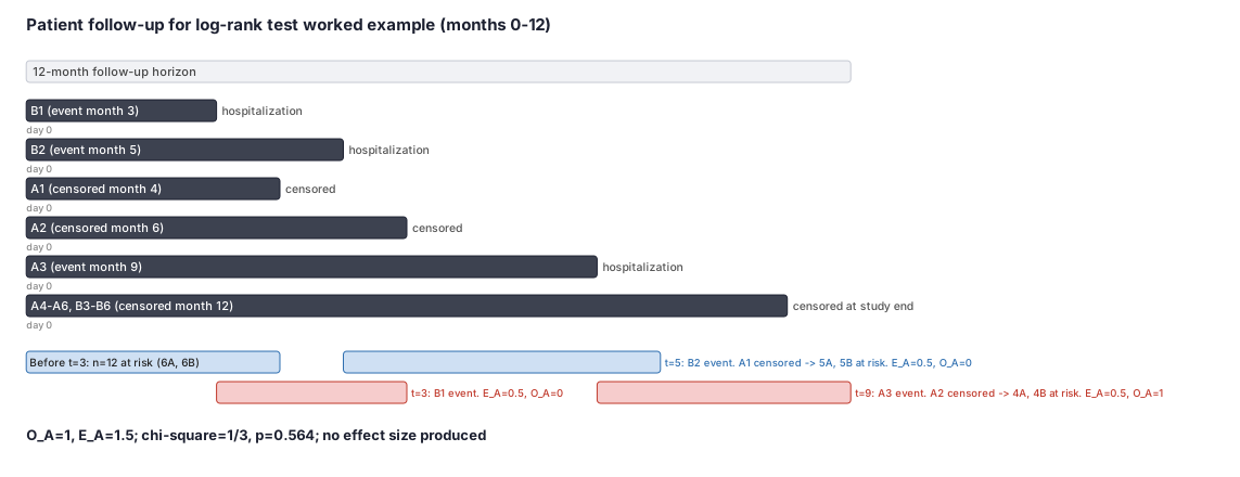
From the worked example: 6 biologic-treatment patients (Group A) and 6 standard-care patients (Group B) followed for up to 12 months. Three event times occurred: month 3 (B1 hospitalized), month 5 (B2 hospitalized), and month 9 (A3 hospitalized). The observed and expected counts sum to O_A = 0 + 0 + 1 = 1 and E_A = 0.5 + 0.5 + 0.5 = 1.5, with total variance V = 0.75. chi-square = 0.25 / 0.75 = 1/3 ≈ 0.333, 1 df, p ≈ 0.564.

(1) Formal interpretation. The log-rank test does not reject the null hypothesis that the biologic and standard-care groups share equal survival functions (chi-square with 1 df ≈ 0.333, p ≈ 0.564). Under repeated sampling from populations with identical hazard functions, a test statistic this extreme or more extreme would occur approximately 56% of the time by chance. Failure to reject does not imply equal survival; the study has only 3 total events and is severely underpowered. The sum O_A - E_A = -0.5 indicates Group A experienced fewer hospitalizations than expected under the null — directionally consistent with biologic benefit — but the variance is large relative to this deviation. No effect size can be read from the test statistic alone: the HR and median survival require a separate Cox model and Kaplan-Meier estimator on the same data.

(2) Practical interpretation. Group A (biologic) had 1 hospitalization while Group B (standard care) had 2, over a 12-patient 12-month illustration. In practice, a time-to-event study with 3 total events provides essentially no inferential value; adequate power for a log-rank test typically requires 50–200 events depending on the expected HR. The log-rank result must be accompanied by a Cox-derived HR with confidence interval (here approximately 0.4, with a very wide CI spanning near-zero to several-fold due to sample size) and Kaplan- Meier median survival estimates. A payer or HTA reviewer needs to know whether the biologic provides, say, 2 additional hospitalization-free months — and that requires an RMST difference or median comparison, not the chi-square alone.

Worked example

Scenario

A 12-month observational follow-up study compares time to first hospitalization in 6 patients receiving a biologic treatment (Group A) versus 6 patients receiving standard care (Group B). One biologic patient transferred to another facility (censored at month 4) and another left the study area (censored at month 6). Two standard-care patients were hospitalized, at months 3 and 5 respectively. One biologic patient was hospitalized at month 9. All remaining patients reached the 12-month study end without a hospitalization. We apply the log-rank test to determine whether the survival curves differ.

Dataset

Per-patient time-to-event data. time_months = months from study entry to hospitalization or last follow-up; status = 1 if hospitalized (event), 0 if censored (transferred care or reached 12-month study end without event).

Steps

• Identify the distinct event times: months 3, 5, and 9 (the three months at which at least one hospitalization occurred). Censored exit times (4, 6, 12) are NOT event times — they reduce the risk set but do not contribute observed events.

• Month 3: At-risk biologic = 6 (A1 is still in the study at month 3), at-risk standard = 6. Total at risk n = 12, events d = 1 (B1 hospitalized). Expected events for biologic group: 6/12 * 1 = 0.5. Observed events in biologic group: 0. Contribution to (O - E): 0 - 0.5 = -0.5.

• Month 5: A1 was censored at month 4, so biologic group now has 5 at risk. B1 had the event at month 3, so standard group has 5 at risk. Total n = 10, events d = 1 (B2 hospitalized). Expected for biologic: 5/10 * 1 = 0.5. Observed: 0. Contribution: -0.5.

• Month 9: A2 was censored at month 6, so biologic group now has 4 at risk. B1 and B2 both had events, so standard group has 4 at risk. Total n = 8, events d = 1 (A3 hospitalized). Expected for biologic: 4/8 * 1 = 0.5. Observed: 1. Contribution: 1 - 0.5 = 0.5.

• Sum the observed and expected counts across all three event times. Total observed in biologic: 0 + 0 + 1 = 1. Total expected in biologic: 0.5 + 0.5 + 0.5 = 1.5. Difference: 1 - 1.5 = -0.5. The biologic group had fewer hospitalizations than expected under the null — directionally consistent with a treatment benefit.

• Compute the variance V_j at each event time using the hypergeometric variance formula V_j = n_A n_B d (n - d) / (n n (n - 1)). At month 3 with n=12, n_A=6, n_B=6, d=1: V = 6 6 1 11 / (144 11) = 0.25. At month 5 with n=10, n_A=5, n_B=5, d=1: V = 5 5 1 9 / (100 9) = 0.25. At month 9 with n=8, n_A=4, n_B=4, d=1: V = 4 4 1 7 / (64 * 7) = 0.25. Total variance: 0.25 + 0.25 + 0.25 = 0.75.

• Compute the log-rank test statistic. chi-square = (O - E) squared divided by V. (O - E) = -0.5; (O - E) squared = 0.25; chi-square = 0.25 / 0.75 = 1/3, approximately 0.333 on 1 degree of freedom, giving p approximately 0.564. Fail to reject H0 — but this example has only 3 total events and is illustrative, not powered for inference.

• The log-rank test returns no effect size. To report the magnitude of the difference, fit a Cox proportional hazards model on the same data (yielding a crude HR with 95% CI) and compute the Kaplan-Meier median hospitalization-free survival for each group. In a real study, always pair the log-rank p-value with these companion measures.

Result

O_A = 0 + 0 + 1 = 1. E_A = 0.5 + 0.5 + 0.5 = 1.5. Difference: 1 - 1.5 = -0.5. Total variance V = 0.25 + 0.25 + 0.25 = 0.75. chi-square = 0.25 / 0.75 = 1/3 ≈ 0.333, 1 df, p ≈ 0.564. Group A (biologic) observed fewer hospitalizations than expected (1 vs 1.5), Group B (standard) observed more (2 vs 1.5). The log-rank test does not reject equal survival (p ≈ 0.564); the study has only 3 events — inadequate power. No effect size is produced by the log-rank; pair with HR and Kaplan-Meier medians.

Timeline Spec

Title

Patient follow-up for log-rank test worked example (months 0-12)

Window

End Day

12

Label

12-month follow-up horizon

Events

• Label

  B1 (event month 3)

  Length Days

  3

  Quantity

  hospitalization

• Label

  B2 (event month 5)

  Length Days

  5

  Quantity

  hospitalization

• Label

  A1 (censored month 4)

  Length Days

  4

  Quantity

  censored

• Label

  A2 (censored month 6)

  Length Days

  6

  Quantity

  censored

• Label

  A3 (event month 9)

  Length Days

  9

  Quantity

  hospitalization

• Label

  A4-A6, B3-B6 (censored month 12)

  Length Days

  12

  Quantity

  censored at study end

Spans

• Kind

  followup

  End Day

  3

  Label

  Before t=3: n=12 at risk (6A, 6B)

• Kind

  gap

  Start Day

  3

  End Day

  5

  Label

  t=3: B1 event. E_A=0.5, O_A=0

• Kind

  followup

  Start Day

  5

  End Day

  9

  Label

  t=5: B2 event. A1 censored -> 5A, 5B at risk. E_A=0.5, O_A=0

• Kind

  gap

  Start Day

  9

  End Day

  12

  Label

  t=9: A3 event. A2 censored -> 4A, 4B at risk. E_A=0.5, O_A=1

Result

Label

O_A=1, E_A=1.5; chi-square=1/3, p=0.564; no effect size produced

Value

0.333

Runnable example

import pandas as pd
from lifelines.statistics import logrank_test, multivariate_logrank_test
from lifelines import KaplanMeierFitter, CoxPHFitter

# ── Worked-example dataset: 12 patients, 12-month follow-up ──────────────────
data = pd.DataFrame({
    'patient_id': ['A1','A2','A3','A4','A5','A6','B1','B2','B3','B4','B5','B6'],
    'group':      ['biologic']*6 + ['standard']*6,
    'time':       [4, 6, 9, 12, 12, 12,  3,  5, 12, 12, 12, 12],
    'event':      [0, 0, 1,  0,  0,  0,  1,  1,  0,  0,  0,  0],
})

grp_a = data[data.group == 'biologic']
grp_b = data[data.group == 'standard']

# ── 1. Standard (unweighted) log-rank test ────────────────────────────────────
lr = logrank_test(
    grp_a['time'], grp_b['time'],
    event_observed_A=grp_a['event'],
    event_observed_B=grp_b['event'],
)
lr.print_summary()
print(f"Log-rank chi-square: {lr.test_statistic:.4f}")
print(f"p-value:             {lr.p_value:.4f}")
print("NOTE: the log-rank test returns no effect size.")
print("      Always report HR and KM medians alongside the p-value.\n")

# ── 2. Kaplan-Meier medians (paired effect estimate) ─────────────────────────
for grp, subset in data.groupby('group'):
    kmf = KaplanMeierFitter()
    kmf.fit(subset['time'], event_observed=subset['event'], label=grp)
    print(f"  {grp}: KM median hospitalization-free survival = "
          f"{kmf.median_survival_time_} months")

# ── 3. Cox HR (paired effect estimate) ───────────────────────────────────────
cph = CoxPHFitter()
data_cox = data.copy()
data_cox['biologic'] = (data_cox['group'] == 'biologic').astype(int)
cph.fit(data_cox[['time','event','biologic']], duration_col='time', event_col='event')
cph.print_summary()

# ── 4. Wilcoxon-Gehan weighted log-rank (emphasizes early differences) ────────
lr_wt = logrank_test(
    grp_a['time'], grp_b['time'],
    event_observed_A=grp_a['event'],
    event_observed_B=grp_b['event'],
    weightings='wilcoxon',    # rho=1, gamma=0 — weights by risk-set size
)
print(f"\nWilcoxon-Gehan log-rank p: {lr_wt.p_value:.4f}")

# ── 5. Fleming-Harrington G(0,1) — emphasizes late differences (IO context) ──
lr_fh = logrank_test(
    grp_a['time'], grp_b['time'],
    event_observed_A=grp_a['event'],
    event_observed_B=grp_b['event'],
    weightings='fleming-harrington',
    p=0, q=1,    # G(rho=0, gamma=1): down-weights early null period
)
print(f"Fleming-Harrington G(0,1) log-rank p: {lr_fh.p_value:.4f}")
print("Use G(0,1) in oncology when delayed treatment effects are expected.")
print("MUST be pre-specified; post-hoc weight selection inflates type-I error.\n")

# ── 6. Stratified log-rank (add a discrete confounder stratum) ───────────────
# In a real study, 'stage' would be a baseline disease-severity variable.
data['stage'] = ['I','II'] * 6
results_mv = multivariate_logrank_test(
    data['time'], data['group'], data['event']
)
print(f"Multivariate log-rank across groups: p = {results_mv.p_value:.4f}")

library(survival)

# ── Worked-example dataset ──────────────────────────────────────────────────
df <- data.frame(
  patient_id = c('A1','A2','A3','A4','A5','A6','B1','B2','B3','B4','B5','B6'),
  group      = c(rep('biologic', 6), rep('standard', 6)),
  time       = c(4, 6, 9, 12, 12, 12,  3,  5, 12, 12, 12, 12),
  event      = c(0, 0, 1,  0,  0,  0,  1,  1,  0,  0,  0,  0)
)

# ── 1. Standard (unweighted) log-rank test ──────────────────────────────────
sd <- survdiff(Surv(time, event) ~ group, data = df)
print(sd)
# survdiff prints: O (observed), E (expected), and chi-square
# Derive the two-sided p-value:
logrank_p <- 1 - pchisq(sd$chisq, df = 1)
cat(sprintf("Log-rank chi-square: %.4f\n", sd$chisq))
cat(sprintf("p-value (1 df):       %.4f\n", logrank_p))
cat("NOTE: survdiff returns no HR. Compute Cox HR separately.\n\n")

# ── 2. Kaplan-Meier medians (paired effect estimate) ────────────────────────
km_fit <- survfit(Surv(time, event) ~ group, data = df)
print(summary(km_fit)$table[, c('records','events','median','0.95LCL','0.95UCL')])

# ── 3. Cox proportional hazards HR ──────────────────────────────────────────
cox_fit <- coxph(Surv(time, event) ~ group, data = df)
summary(cox_fit)     # HR, 95% CI, and Wald/likelihood-ratio tests

# ── 4. Wilcoxon-Gehan weighted log-rank (rho = 1, early emphasis) ───────────
sd_wt <- survdiff(Surv(time, event) ~ group, data = df, rho = 1)
cat(sprintf("Wilcoxon-Gehan (rho=1) chi-sq: %.4f, p: %.4f\n",
            sd_wt$chisq, 1 - pchisq(sd_wt$chisq, df = 1)))
cat("rho=1 weights each event time by the current risk-set size.\n")
cat("Use when early differences are the scientific hypothesis.\n\n")

# ── 5. Stratified log-rank (adjusts for a discrete confounder) ───────────────
# Artificial stratification variable to illustrate the syntax:
df$stage <- rep(c('I','II'), 6)
sd_strat <- survdiff(Surv(time, event) ~ group + strata(stage), data = df)
cat(sprintf("Stratified log-rank chi-sq: %.4f, p: %.4f\n",
            sd_strat$chisq, 1 - pchisq(sd_strat$chisq, df = 1)))
cat("Stratified log-rank sums within-stratum (O-E) contributions,\n")
cat("removing between-stratum baseline hazard variation.\n")