Lead-Time and Length Bias in RWE
A pair of related detection-timing biases in which (1) earlier disease detection mechanically lengthens the apparent survival time measured from diagnosis without changing the date of death (lead-time bias), and (2) periodic or opportunistic detection (screening, imaging surveillance, incidental diagnosis) systematically over-samples slower-growing, better-prognosis disease because it sits in a detectable state longer (length bias) — together making an earlier-detected or more intensively surveilled RWE cohort look healthier than a comparator even when there is no true difference in treatment effect or screening benefit. The two mechanisms are not interchangeable — lead-time bias holds the underlying disease identical for a given patient and shifts only the measurement clock, while length bias changes *which* patients end up in the detected cohort — the two groups' realized mix of tumor aggressiveness differs by construction, so a shared start date alone cannot remove it.
On this page
Lead-time bias happens when a disease is found earlier than it otherwise would have been — say, by a screening test — which makes a patient look like they lived longer after diagnosis, even though the actual day they died never moved.
Length bias is a companion problem, but it works differently: periodic checks like screening are much better at catching slow-growing, less dangerous disease than fast-growing disease, because slow disease sits in a findable window for years while fast disease can appear and cause symptoms between two checks and get missed. That means a screened group isn't just measured differently — it is actually made up of a milder mix of disease than an unscreened group, even before anyone starts treatment.
Together, these two effects can make an early-detected or heavily-monitored group look healthier than a comparison group even when there is no true difference in how well the treatment works. Comparing people from a start date that isn't distorted by how or when they were found — instead of the date a diagnosis was written down — removes the lead-time part of the distortion, but it does nothing about the fact that the two groups still contain a different mix of disease severity; fixing that requires accounting for how each patient was found in the first place, not just when.
The mechanism: two distinct distortions that are almost always discussed together
Lead-time bias and length bias both arise from how and when disease is detected, and both inflate apparent survival independent of any true treatment or screening benefit — but they operate through different causal paths, and conflating them leads to the wrong fix.
Lead-time bias is purely a clock-placement artifact. Apparent survival is measured as (date of death) minus (date of diagnosis). If a screening test, an incidental imaging finding, or more frequent surveillance moves the diagnosis date earlier by an interval L (the "lead time"), apparent survival grows by exactly L — even if the disease's natural history, the treatment given, and the actual date of death are completely unchanged.
A widely used pedagogical illustration in the screening-evaluation literature makes this concrete with hypothetical identical twins sharing the same tumor: one is screen-detected 12 months before symptoms would have appeared, the other is detected the usual way, symptomatically. Both die on the same calendar date. The screen-detected twin's chart shows 12 months of "extra" survival that reflects nothing but an earlier start line.
Hutchison & Shapiro (1968) is the foundational quantitative source for lead-time bias itself — using outcome data from the HIP (Health Insurance Plan) breast-cancer screening trial to estimate the actual magnitude of lead time gained by screening — establishing the same earlier-clock-start mechanism the twins device teaches, though the twins illustration itself is a later pedagogical simplification rather than a verbatim example from their paper.
Length bias is a selection artifact, not a clock artifact. Any detection process that samples disease at a point in time — a screening round, a surveillance scan, an incidental finding — is more likely to catch a case with a long detectable-but-asymptomatic phase (a long "sojourn time") than a case with a short one, for the same reason a slow-moving object is easier to photograph than a fast one.
Aggressive, fast-growing disease tends to become symptomatic and get diagnosed between screening rounds — an "interval" case — rather than being caught by the screen itself. The result is that a screen-detected (or otherwise periodically detected) cohort is enriched for indolent, better-prognosis disease relative to a symptomatically detected cohort, quite apart from any lead time.
A simplified model that isolates the mechanism makes this quantitative: with a fixed screening interval `I`, a deterministic sojourn time `t` (the length of the detectable-but- asymptomatic phase), perfect test sensitivity, and disease onset uniformly phased relative to the screening schedule, the probability that a given case is caught by a screen (rather than presenting as an interval cancer between screens) is `min(t / I, 1)` — a case with a sojourn time at or beyond the screening interval is essentially certain to be caught by some round, while a case with a shorter sojourn time is caught only if its detectable window happens to overlap a scheduled screen.
Because detection probability rises with sojourn time, long-sojourn (indolent) disease is disproportionately represented among screen-detected cases. The fuller statistical machinery for estimating a real sojourn-time distribution (not just this single-value illustration) from actual multi-round screening data — treating sojourn time as a random variable and using the pattern of screen-detected versus interval cases across rounds to back out its distribution — was formalized by Walter & Day (1983).
Core conceptual distinction and why it matters for the fix
Lead-time bias inflates survival for every early-detected patient by the same underlying mechanism (an earlier clock start), which is why it disappears entirely if the outcome is measured from a shared anchor common to all patients (e.g., population-level mortality per person invited to screening, or a treatment-initiation date common to both arms) instead of from the diagnosis date.
It is not, however, fixed by subtracting a single population-average lead time from every patient's observed survival after the fact: lead time varies systematically with tumor aggressiveness (fast tumors have short lead times, slow tumors have long ones — see "When NOT to use" below), so a blanket subtraction under- and over-corrects different patients simultaneously rather than restoring comparability. The only complete fix is realigning the clock itself, not adjusting the resulting survival number.
Length bias changes who is in the cohort — it cannot be fixed by shifting a clock at all, because the problem is compositional: the detected group contains a different mix of disease aggressiveness than the source population.
Restriction/stratification by detection route can reduce between-group imbalance in that mix, but the only way to remove length bias itself is a design that samples disease independent of its sojourn time (e.g., comparing outcomes among everyone eligible for screening rather than only those diagnosed by screening) — see the ranked fixes below for the distinction between reducing imbalance and removing the bias.
In real screening evaluations and RWE detection-timing comparisons the two nearly always co-occur and compound in the same direction (toward an inflated apparent benefit of earlier/more intensive detection), which is why regulators and methodologists treat them as a paired family.
A closely related third phenomenon, stage migration (the Will Rogers phenomenon), is not a survival-clock or a sampling artifact but a reclassification artifact: when a more sensitive staging technology finds previously invisible low-volume disease, patients migrate from an earlier to a later stage category. Both categories then show improved stage-specific survival — the earlier stage loses its worst cases, the later stage gains relatively better ones — even though no individual patient's outcome changed and overall survival is flat (Feinstein, Sosin & Wells, 1985).
It belongs in this entry because it produces the same signature as lead-time/length bias (apparent improvement with no true underlying change) and is driven by the same root cause: a change in detection capability.
RWE manifestations
- rwPFS vs. trial PFS — assessment-time (interval-censoring) bias, a cousin of classic lead-time bias rather than the same mechanism. Clinical trials mandate protocol-driven scans on a fixed schedule (e.g., every 6–8 weeks); routine real-world imaging is sparser, irregular, and driven by clinical judgment. Progression that occurred biologically on day 42 may not be recorded until day 90 in claims/EHR data simply because no scan happened sooner — this is assessment-time bias (a form of interval censoring on the progression event itself), distinct from the diagnosis-earlier- than-symptoms lead-time mechanism described above, though the two are discussed together because both stem from unequal detection timing. A discrete-event-simulation study calibrated to real EHR imaging-frequency patterns found that differential imaging-assessment timing between compared treatment groups biases the estimated PFS hazard ratio, with the size (and direction) of the bias depending on how differently the groups are scanned and how fast the disease progresses (Adamson et al., 2022) — real but conditional, not a fixed "rwPFS always runs long" rule. Whether a given rwPFS estimate runs systematically longer or shorter than a comparably defined trial PFS depends on the progression-ascertainment rule used (RECIST-like, radiology-anchored, clinician-anchored — these approaches can themselves differ from each other by under a month even within the same EHR source; Griffith et al., 2019) and on the specific comparison; it should be checked empirically, not assumed in either direction. See `real-world-progression-rwpfs-rwe`.
- Single-arm external controls with mismatched index dates — two mechanistically distinct failure modes. A single-arm trial's OS/PFS clock typically starts at treatment initiation. An external control built from a registry or claims source often can only be reliably anchored at an earlier milestone — initial diagnosis or metastatic diagnosis — because that is what the source data captures cleanly. (1) External control anchored earlier than the trial (classic lead time). If the control's clock starts earlier than the trial arm's and both experience the same underlying disease course, the control gains lead time and shows the longer apparent survival — this biases the comparison against the treatment (it understates, or can even reverse the sign of, a true trial-arm benefit), not the "trial looks artificially good" story it is sometimes assumed to produce. (2) Trial arm delayed behind a shared milestone the external control isn't held to (immortal/guarantee time). When trial patients must first survive from an earlier milestone (e.g., relapse) to treatment initiation before their trial clock starts, but the external-control cohort is not required to survive an analogous interval, the trial arm instead gains immortal time and looks artificially better — the reverse direction from (1). This was the actual mechanism the FDA identified as a major bias source in the October 2022 Oncologic Drugs Advisory Committee (ODAC) review of the externally controlled ¹³¹I-omburtamab submission (BLA 761176, single-arm Study 03-133 vs. a German-registry external control): trial patients had to survive a median 3.1 months from the start of their last post-relapse treatment modality to omburtamab initiation, while external controls faced no analogous requirement — 24 of 79 external-control patients who received comparable post-relapse therapy died within that 3.1-month window (Le Coënt et al., 2026, reporting the FDA's own account of the case). See `immortal-time-bias-handling` for the guarantee-time mechanism and `rare-disease-external-controls-rwe` for the full external-control design.
- Screening-detected vs. symptom-detected cohorts. Any RWE comparative-effectiveness study that pools screen-detected and symptom-detected patients — common in claims/registry cancer cohorts where detection route is not a clean coded field — will show the screen-detected subgroup living longer from diagnosis, independent of any treatment difference, from the combined action of lead time and length bias.
- Stage migration across diagnostic eras or data sources. A time-trend comparison of stage- specific survival across calendar periods (before/after PET-CT or liquid-biopsy adoption), or a pooled comparison across data sources with different staging intensity (e.g., an EHR cohort with routine molecular staging vs. a claims/registry cohort relying on coarser ICD-coded stage), will show spurious within-stage improvement or decline driven entirely by reclassification.
Fixes, ranked
[1] Compare outcomes anchored to a shared, detection-independent event in the full eligible population (gold standard, when feasible). In a true screening evaluation this means comparing mortality per person invited to screening (or per person in the source population) rather than survival from the date of diagnosis — every person contributes follow-up from the same clock regardless of whether, or when, they were ever diagnosed. This eliminates lead-time bias by construction and eliminates length bias because the comparison no longer conditions on having been detected at all.
Cost: requires population-level (not diagnosis-cohort) data and is rarely available outside dedicated screening trials or registries with denominator data. [2] Index-date alignment to a shared, detection-route-independent anchor. When the population-level comparison is not feasible (the typical RWE/external-control situation), anchor both arms to the closest available analog of the same clinical decision point — e.g., treatment initiation for both the trial arm and the external control, not diagnosis — rather than to whichever date each data source happens to capture most easily. See `time-zero-index-date-alignment-rwe`.
This is the primary, regulator-facing fix for external-control and comparative-effectiveness lead time.
[3] Landmark analysis — a general sensitivity check, not a lead-time fix. Restricting to patients alive and under observation at a fixed landmark does not, by itself, correct lead-time bias: if the landmark is measured from each arm's own still-mismatched native index date, the disparate clocks are preserved and only the earliest, most-distorted follow-up window is discarded; if it is measured from an already-aligned shared anchor, fix [2] is doing the real work and the landmark step adds nothing to it beyond a stability check.
Either way, landmarking additionally conditions the analysis on survival to the landmark, which changes the study population to those who survived long enough to be observed and can introduce its own survivor-selection distortion. Use it as a supplementary robustness check for early-follow-up instability generally, not as a substitute for index-date alignment, and it does nothing for length bias regardless. See `landmark-analysis`.
[4] Restrict or stratify by detection route. When pooling screen-detected and symptom-detected (or incidentally-detected) patients cannot be avoided, treat detection route as an explicit stratification variable or exclusion criterion rather than analyzing the pooled cohort as if detection route were exchangeable. This reduces between-group imbalance in detection-route mix; it does not, by itself, remove the length-bias-driven case-mix distortion that remains within each detection-route stratum relative to the full source population — only a population-anchored design (fix [1]) does that.
[5] Report and, where possible, model the assessment-interval distribution for rwPFS. Publish the actual inter-scan interval alongside rwPFS, and prefer symptomatic/clinical-progression capture rules or sensitivity analyses across assumed interval lengths over presenting a single rwPFS number as directly comparable to a trial's protocol-driven PFS.
Pros, cons, and trade-offs
- Population-anchored mortality comparison vs. index-date alignment. The population comparison is the only approach that removes both biases completely, but it requires data most RWE studies do not have (an enumerated source population with complete follow-up regardless of diagnosis status). Index-date alignment is achievable with typical claims/EHR/registry data and removes the lead-time component when a genuinely comparable anchor exists in both arms, but it cannot fix length bias if the comparator groups differ systematically in how they were detected. Prefer the population comparison whenever a true screening/detection-policy question is being asked with denominator data; prefer index-date alignment for comparative-effectiveness and external-control questions built from diagnosed/treated cohorts.
- Index-date alignment vs. landmark analysis. Alignment is the more complete fix because it actually changes what the clock measures for every patient; landmarking is simpler to implement and requires no judgment about which anchor is "truly" comparable, but — unless applied after alignment — it does not correct a mismatched clock at all, only discards the earliest, most- distorted person-time and events, and it conditions on survival to the landmark, introducing its own selection effect. It leaves length bias fully untouched regardless. Prefer alignment as the primary analysis; reserve landmarking for a fast sensitivity check on early-follow-up stability, not as a lead-time remedy in its own right, or for when a comparable alternative anchor genuinely does not exist in the data.
- Detection-route restriction vs. leaving the pooled cohort intact. Restriction reduces the between-group imbalance in detection-route mix — it stops one arm from being disproportionately screen-detected relative to the other — but it does not eliminate length bias itself: within a screen-detected stratum, cases remain enriched for indolent, long-sojourn disease relative to the full source population, and no amount of stratification recovers the disease-mix comparability of a true population-anchored design. It can also shrink an already-modest RWE sample and requires a codable or chart-confirmable detection-route variable, which is often unavailable or noisy in claims data. Prefer restriction whenever detection route materially differs across the groups being compared and can be ascertained, treating it as a partial mitigation of route imbalance rather than a cure for length bias; accept the pooled cohort only with an explicit acknowledgment that length bias is uncontrolled either way.
When NOT to use — and when the "fix" is actively misleading
- Applying a mean-lead-time subtraction as a blanket correction. Lead time varies by tumor aggressiveness (fast tumors have short lead times, slow tumors have long ones), so subtracting a single population-average lead time from every patient's survival both under-corrects the indolent cases and over-corrects the aggressive ones — it does not restore comparability and should not be presented as if it does.
- Treating index-date alignment as a fix for length bias. Aligning the clock only addresses when follow-up starts; it does nothing about which patients were selected into the detected group in the first place. A perfectly time-zero-aligned comparison between a screen-detected and a symptom-detected cohort still carries the full length-bias distortion.
- Ignoring stage migration when comparing survival across calendar eras or data sources with different staging technology. A naive "outcomes have improved over time" or "data source A shows better stage-specific survival than data source B" claim, made without accounting for staging-era or staging-intensity differences, risks attributing a pure reclassification artifact to a real clinical improvement.
- Using landmark analysis alone as if it solved detection-timing bias. Landmarking does not itself correct a mismatched index date — a diagnosis-anchored landmark still starts each arm's clock at a different point, it only discards the earliest window. It conditions on survival to the landmark (a selected population) and leaves length bias fully intact — it is a general sensitivity check, not a primary remedy, for this bias family.
Data-source operational depth
- Claims (FFS): Detection route is rarely a discrete field. Approximate screen-detection by the presence of a screening-procedure code (mammography, low-dose CT, colonoscopy) in the lookback window immediately preceding the diagnosis code, versus a first-presentation pattern via an ED or urgent symptomatic encounter. Stage is often absent or crudely proxied; treat any claims-derived stage-stratified trend across calendar years with caution because staging intensity (more frequent imaging, newer CPT codes for advanced imaging) changes over time within the same claims stream.
- EHR: Structured screening orders and radiology/pathology report text can flag screen-detected vs. symptomatic presentation more reliably than claims codes; validate against a linked tumor registry's mode-of-detection field only when the specific registry in use actually carries one (see the Registry note below — SEER does not). Scan-interval data (the actual gap between imaging studies) is directly observable in EHR order/result timestamps and should be reported alongside any rwPFS estimate rather than assumed to match a trial's protocol schedule.
- Registry: Cancer registries (e.g., SEER) are the primary source of denominator-level population data needed for the gold-standard population-based mortality-rate comparison (mortality per person in the source/catchment population) in fix [1], and they are usually the best available source for stage at diagnosis. SEER carries no screening-invitation or eligibility records, so it cannot by itself support the "per person invited to screening" framing of fix [1] — that version requires a screening-program registry/trial or linkage to program participation records, not SEER alone. Registries are also not, by default, a reliable source for detection route: SEER's "diagnostic confirmation" field records how the malignancy was confirmed (histology, cytology, direct visualization, imaging, or clinical diagnosis alone) — not what prompted the workup that led to diagnosis — so it cannot substitute for a screen-detected-vs- symptomatic flag. Restricting or stratifying by detection route from registry data requires either a registry with a genuine mode-of-detection field (some population-based or screening-program-linked registries outside SEER carry one), linkage to the screening program's own participation records, or validated chart abstraction; absent one of those, treat detection route as unmeasured in a SEER-only analysis rather than approximating it from diagnostic-confirmation codes. Registries are typically weak for the fine-grained treatment-date data needed to build a treatment-anchored index date for external controls — link to claims/EHR for that anchor when possible.
- Linked: Linked claims-EHR-registry data gives the best combination of a reliable diagnosis/stage date (registry), a reliable treatment-initiation date (claims/EHR), and enough clinical detail to approximate detection route — the recommended substrate for building an index-date-aligned external control or a detection-route-restricted comparison. Reconcile diagnosis-date discrepancies across sources before choosing the anchor; a registry diagnosis date and a claims first-treatment-related- code date can differ by months.
Worked example (hypothetical twins)
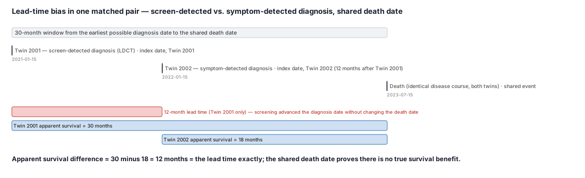
Two patients with molecularly identical, indolent lung tumors would — absent any screening — both first become symptomatic and be diagnosed on 2022-01-15, and both die of the same disease course on 2023-07-15. Twin 2001 undergoes low-dose CT screening, which finds the tumor on 2021-01-15, twelve months before it would have become symptomatic. Twin 2002 receives no screening and is diagnosed the usual way, on 2022-01-15.
A naive analysis computing "months survived since diagnosis" reports Twin 2001 at 30 months (2021-01-15 to 2023-07-15) and Twin 2002 at 18 months (2022-01-15 to 2023-07-15) — a 12-month apparent advantage for the screened twin. But both twins die on the identical calendar date. The entire 12-month gap is lead time: screening moved the diagnosis date earlier without moving the death date at all.
Because these are matched twins with truly identical tumor biology, the example isolates lead time from length bias — in a real screened population, most of the twins that got detected early instead of not-at-all would additionally, on average, have slower-growing tumors than the ones missed between screens, adding a length-bias inflation on top of this lead-time inflation.
Interpreting the output
In the worked twin example, Twin 2001 (screen-detected) shows 30 months of apparent survival and Twin 2002 (symptom-detected) shows 18 months, a 12-month difference.
(1) Formal interpretation. Apparent survival is calculated as death date minus diagnosis date for each twin. Because the twins are constructed to share an identical death date (2023-07-15) and an identical underlying disease course, the entire 30-versus-18-month gap is attributable to the 12-month difference in diagnosis date — the lead time — with zero contribution from any true difference in disease progression or treatment effect. The true survival benefit of screening in this example is exactly zero months.
(2) Practical interpretation. If a claims- or registry-based analyst compared "years survived since diagnosis" between a screened cohort and an unscreened cohort without accounting for lead time, a result structurally identical to this twin comparison would be read as "screening extends survival by a year" — a conclusion that could drive a screening-program investment decision or a real-world comparative-effectiveness claim that is entirely an artifact of when the diagnosis was recorded, not of any clinical benefit.
The correct comparison anchors both twins to a shared clock (e.g., calendar time, or time since a shared eligibility date) rather than to each twin's own diagnosis date.
Decision diagram
flowchart LR
  Twin1["Twin 2001: screen-detected\ndiagnosis 2021-01-15"]
  Twin2["Twin 2002: symptom-detected\ndiagnosis 2022-01-15\n(12 months later)"]
  LT["12-month lead time\n(identical tumor biology,\nno true survival change)"]
  Death["Shared death date\n2023-07-15"]
  Naive["Naive comparison:\n'survival since diagnosis'\nTwin 2001 = 30mo, Twin 2002 = 18mo"]
  Wrong["Misread as a\n12-month survival benefit\nof screening"]

  Twin1 -->|earlier clock start| LT
  Twin2 -->|later clock start| LT
  Twin1 --> Death
  Twin2 --> Death
  Twin1 & Twin2 -->|measured from each\ntwin's own diagnosis date| Naive
  Naive -->|if not corrected| Wrong
  style LT fill:#ffe0cc,stroke:#cc6600
  style Wrong fill:#ffcccc,stroke:#cc0000
  style Death fill:#ccffcc,stroke:#00aa44
flowchart TD
  Q{What is being compared?} -->|Survival/PFS from diagnosis\nor imaging across groups\nwith different detection timing| M1{Is population-level\ndenominator data\navailable, e.g. a true\nscreening evaluation?}
  M1 -->|Yes| POP[Gold standard: compare mortality\nper person in the source population,\nnot survival from diagnosis]
  M1 -->|No: comparative-effectiveness\nor external-control design| ALIGN[Index-date alignment:\nanchor all arms to the same\ntreatment-initiation analog]
  ALIGN --> Feasible{Comparable anchor\nobservable in all arms?}
  Feasible -->|Yes| Done[Primary analysis on\naligned index date]
  Feasible -->|No| LAND[Landmark analysis as a\nsensitivity check only --\ndoes not fix length bias]
  Q -->|Screen-detected vs.\nsymptom-detected cohorts\npooled together| RESTRICT[Restrict or stratify\nby detection route]
  Q -->|Stage-specific survival trend\nacross eras or data sources| STAGE[Check for stage migration\n/ Will Rogers phenomenon:\nstratify by staging era/technology]
POP & Done & LAND & RESTRICT & STAGE --> REPORT[Report both naive and\ncorrected estimates;\nstate which bias each fix addresses]Worked example
Scenario
Two patients have molecularly identical, indolent lung tumors with an identical natural history. Without screening, both would first become symptomatic and be diagnosed on 2022-01-15, and both would die of the same disease course on 2023-07-15. Twin 2001 undergoes low-dose CT screening, which finds the tumor on 2021-01-15 — twelve months before it would have caused symptoms. Twin 2002 receives no screening and is diagnosed the usual way, when symptoms appear. A naive analyst compares "months survived since diagnosis" between the two.
Dataset
Event-level records for the two twins, as an analyst would see them in a registry or EHR extract — diagnosis and death events with dates, no pre-computed survival column.
| person_id | event_date | event_type | detection_route |
|---|---|---|---|
| 2001 | 2021-01-15 | Diagnosis (lung cancer) | Screen-detected (LDCT) |
| 2001 | 2023-07-15 | Death | |
| 2002 | 2022-01-15 | Diagnosis (lung cancer) | Symptom-detected |
| 2002 | 2023-07-15 | Death |
Steps
Result
- Label
Apparent survival — screen-detected twin = 30 months; symptom-detected twin = 18 months; difference = 12 months, exactly equal to the lead time. True survival benefit = 0 months, since the death date is identical for both twins.
- Value
12
Trade-offs
Runnable example
Computes naive (diagnosis-anchored) apparent survival for the twin worked example, then demonstrates the index-date-alignment fix for a single-arm-trial external-control comparison by recomputing survival from a shared treatment-anchor date instead of each arm's native index date.
import pandas as pd

# ── Twin worked example: naive apparent survival from diagnosis ─────────────────────────
twins = pd.DataFrame({
    "person_id": [2001, 2002],
    "detection_route": ["screen-detected", "symptom-detected"],
    "diagnosis_date": pd.to_datetime(["2021-01-15", "2022-01-15"]),
    "death_date": pd.to_datetime(["2023-07-15", "2023-07-15"]),
})
twins["apparent_survival_months"] = (
    (twins["death_date"] - twins["diagnosis_date"]).dt.days / 30.44
).round(1)
print(twins[["person_id", "detection_route", "apparent_survival_months"]])
# Twin 2001 (screen-detected): 29.9 months. Twin 2002 (symptom-detected): 17.9 months.
# (Exact calendar-month arithmetic gives 30 and 18; the day-count/30.44 approximation used
# here is the standard real-data convention and differs by about 0.1 month -- roughly three
# days -- because dividing exact day-counts by a fixed 30.44-day "average month" does not
# reproduce true calendar-month arithmetic for these particular dates.) Both share death_date
# -> the ~12-month gap is lead time, not a survival difference.

# ── External-control index-date alignment fix ───────────────────────────────────────────
def naive_vs_aligned_survival(cohort: pd.DataFrame) -> pd.DataFrame:
    """
    cohort: person_id, arm, diagnosis_date, treatment_start_date (NaT if unobserved),
            death_date.
    Returns both the naive (native index date per arm) and aligned (shared treatment-start
    anchor) apparent survival, so the lead-time gap introduced by anchor-date mismatch is
    visible rather than silently absorbed into the naive comparison.
    """
    df = cohort.copy()
    # Naive: trial arm anchored at treatment_start, external control anchored at diagnosis
    # (the classic mismatch that manufactures apparent lead time for the control arm).
    df["naive_index"] = df["treatment_start_date"].where(
        df["arm"] == "trial", df["diagnosis_date"]
    )
    # Aligned: both arms anchored at the closest available treatment-start analog; rows
    # without an observed treatment_start_date cannot be aligned and are flagged, not
    # silently defaulted back to diagnosis_date.
    df["aligned_index"] = df["treatment_start_date"]
    df["alignable"] = df["aligned_index"].notna()

    df["naive_survival_months"] = (
        (df["death_date"] - df["naive_index"]).dt.days / 30.44
    ).round(1)
    df["aligned_survival_months"] = (
        (df["death_date"] - df["aligned_index"]).dt.days / 30.44
    ).round(1)
    return df

external = pd.DataFrame({
    "person_id": [3001, 3002, 3003],
    "arm": ["trial", "external_control", "external_control"],
    "diagnosis_date": pd.to_datetime(["2020-06-01", "2020-06-01", "2020-06-01"]),
    "treatment_start_date": pd.to_datetime(["2020-07-01", pd.NaT, "2020-08-15"]),
    "death_date": pd.to_datetime(["2022-01-01", "2022-01-01", "2022-01-01"]),
})
result = naive_vs_aligned_survival(external)
print(result[["person_id", "arm", "naive_survival_months",
               "aligned_survival_months", "alignable"]])
# Naive: both external-control rows are anchored at the earlier diagnosis date and show
# 19.0 months vs. the trial arm's 18.0 months -- an apparent ~1-month control "advantage"
# that is pure lead time, not a real survival difference (confirms the control, not the
# trial, is the arm whose apparent survival is inflated by an earlier anchor).
# Aligned: person 3003 has an observed treatment_start_date (2020-08-15) and re-anchors to
# 16.6 months once placed on the same treatment-initiation clock as the trial arm --
# revealing that the naive comparison had the wrong arm looking better: on a shared clock
# the trial arm's 18.0 months now exceeds the aligned control's 16.6 months. Person 3002's
# treatment_start_date is unobserved (registry-only) -> flagged alignable=False rather than
# silently reusing diagnosis_date as a false treatment anchor.
Mirrors the Python twin calculation and the index-date-alignment demonstration using base R Date arithmetic; no external packages required for the core arithmetic.
# ── Twin worked example: naive apparent survival from diagnosis ─────────────────────────
twins <- data.frame(
  person_id        = c(2001, 2002),
  detection_route  = c("screen-detected", "symptom-detected"),
  diagnosis_date   = as.Date(c("2021-01-15", "2022-01-15")),
  death_date       = as.Date(c("2023-07-15", "2023-07-15"))
)
twins$apparent_survival_months <- round(
  as.numeric(twins$death_date - twins$diagnosis_date) / 30.44, 1
)
print(twins[, c("person_id", "detection_route", "apparent_survival_months")])
# Twin 2001: 29.9 months. Twin 2002: 17.9 months. (Exact calendar-month arithmetic gives
# 30 and 18; the day-count/30.44 approximation differs by about 0.1 month -- roughly three
# days -- because dividing exact day-counts by a fixed 30.44-day "average month" does not
# reproduce true calendar-month arithmetic for these particular dates.) Shared death_date
# -> the ~12-month gap is entirely lead time.

# ── External-control index-date alignment fix ───────────────────────────────────────────
naive_vs_aligned_survival <- function(cohort) {
  # cohort: person_id, arm, diagnosis_date, treatment_start_date (NA if unobserved), death_date
  cohort$naive_index <- ifelse(cohort$arm == "trial",
                                as.character(cohort$treatment_start_date),
                                as.character(cohort$diagnosis_date))
  cohort$naive_index <- as.Date(cohort$naive_index)
  cohort$aligned_index <- cohort$treatment_start_date       # NA when unobserved
  cohort$alignable <- !is.na(cohort$aligned_index)

  cohort$naive_survival_months   <- round(as.numeric(cohort$death_date - cohort$naive_index) / 30.44, 1)
  cohort$aligned_survival_months <- round(as.numeric(cohort$death_date - cohort$aligned_index) / 30.44, 1)
  cohort
}

external <- data.frame(
  person_id            = c(3001, 3002, 3003),
  arm                  = c("trial", "external_control", "external_control"),
  diagnosis_date       = as.Date(c("2020-06-01", "2020-06-01", "2020-06-01")),
  treatment_start_date = as.Date(c("2020-07-01", NA, "2020-08-15")),
  death_date           = as.Date(c("2022-01-01", "2022-01-01", "2022-01-01"))
)
result <- naive_vs_aligned_survival(external)
print(result[, c("person_id", "arm", "naive_survival_months",
                  "aligned_survival_months", "alignable")])
# Naive: both external-control rows are anchored at the earlier diagnosis_date and show
# 19.0 months vs. the trial arm's 18.0 months -- an apparent lead-time "advantage" for the
# control, not the trial.
# Aligned: person 3003 has an observed treatment_start_date (2020-08-15) and re-anchors to
# 16.6 months on the same treatment-initiation clock as the trial arm, so the aligned
# comparison (18.0 trial vs. 16.6 control) reverses the naive read. Person 3002's
# treatment_start_date is NA -> flagged alignable=FALSE rather than silently substituting
# diagnosis_date as a false treatment anchor.
Computes naive apparent survival (index = each arm's native date) and an aligned survival (index = treatment_start_date only, with unalignable rows flagged) so the lead-time gap between a diagnosis-anchored and a treatment-anchored comparison is visible in the output rather than absorbed into a single unexamined...
/* work.cohort: person_id, arm ($, "trial" or "external_control"), diagnosis_date,        */
/* treatment_start_date (missing if unobserved), death_date (all SAS date values).        */

data work.aligned;
  set work.cohort;

  /* Naive index: trial arm anchored at treatment start, external control anchored at   */
  /* diagnosis -- the classic mismatch that manufactures apparent lead time for the      */
  /* control arm when the two arms are compared as if their clocks were equivalent.      */
  if arm = "trial" then naive_index = treatment_start_date;
  else naive_index = diagnosis_date;

  /* Aligned index: both arms anchored at the same treatment-start analog; rows without */
  /* an observed treatment_start_date are flagged, never silently defaulted back to      */
  /* diagnosis_date as a false treatment anchor.                                         */
  aligned_index = treatment_start_date;
  alignable = (treatment_start_date ne .);

  naive_survival_months   = (death_date - naive_index) / 30.44;
  aligned_survival_months = (death_date - aligned_index) / 30.44;
  format naive_index aligned_index diagnosis_date treatment_start_date death_date date9.;
run;

proc print data=work.aligned noobs;
  var person_id arm naive_survival_months aligned_survival_months alignable;
run;

/* Naive: external_control's earlier diagnosis-anchored clock inflates its apparent      */
/* survival relative to the trial arm; the gap between naive_survival_months and         */
/* aligned_survival_months for the external_control arm is the manufactured lead time.   */
Citations
- [1]Hutchison GB, Shapiro S. Lead time gained by diagnostic screening for breast cancer. Journal of the National Cancer Institute. 1968;41(3):665-681.
- [2]Walter SD, Day NE. Estimation of the duration of a pre-clinical disease state using screening data. American Journal of Epidemiology. 1983;118(6):865-886.
- [3]Feinstein AR, Sosin DM, Wells CK. The Will Rogers phenomenon: stage migration and new diagnostic techniques as a source of misleading statistics for survival in cancer. New England Journal of Medicine. 1985;312(25):1604-1608.
- [4]Griffith SD, Tucker M, Bowser B, Calkins G, Chang C, Guardino E, Khozin S, Kraut J, You P, Schrag D, Miksad RA. Generating real-world tumor burden endpoints from electronic health record data: comparison of RECIST, radiology-anchored, and clinician-anchored approaches for abstracting real-world progression in non-small cell lung cancer. Advances in Therapy. 2019;36(8):2122-2136.
- [5]Adamson BJS, Ma X, Griffith SD, Sweeney EM, Sarkar S, Bourla AB. Differential frequency in imaging-based outcome measurement: Bias in real-world oncology comparative- effectiveness studies. Pharmacoepidemiology and Drug Safety. 2022;31(1):46-54.
- [6]Huang Bartlett C, Mardekian J, Cotter MJ, Huang X, Zhang Z, Parrinello CM, Bourla AB. Concordance of real-world versus conventional progression-free survival from a phase 3 trial of endocrine therapy as first-line treatment for metastatic breast cancer. PLOS ONE. 2020;15(4):e0227256.
- [7]Le Coënt Q, Rosner GL, Wang MC, Hu C. Index Date Imputation for Survival Analysis in Externally Controlled Trials with Delayed Treatment Initiation. arXiv:2509.14183 (posted 2025-09-17, revised 2026-06-16).